Using ExoMol files

PGOPHER can make use of linelists produced in the ExoMol linelist format, part of the ExoMol project. The way these linelists are structured make it possible to use many of the features of PGOPHER on energy levels and transitions calculated by other programs, to produce energy levels plots, for example, in addition to simulations. For documentation of the format see Jonathan Tennyson, Christian Hill, and Sergei N. Yurchenko AIP Conf. Proc. 1545, 186 (2013) doi: 10.1063/1.4815853.

Simulations using ExoMol files

To produce a simulation first import the .states file into PGOPHER (File, Import, ExoMol File...). This will produce a Manifold object (ExoManifold) containing the states. Then, in the constants window right click on the Manifold produced and select "Add .trans file...", and select the required file. The process can be repeated if there is more than one .trans file. By default, the partition function is calculated by summing over the energy levels in the .states file, but the partition function can be specified as a table of values using an Interpolated Transition Function. To add this, right click on Molecule, Add New..., Interpolated Partition Function and then right click on the Interpolated Partition Function object and select the file. The resulting file will produce simulations in the normal way, allowing the temperature and linewidth to be adjusted and right clicking on any transition will give the underlying quantum numbers.

Fitting to values in ExoMol files

The values in ExoMol files can also be used as input to line position or intensity fitting. To fit to energy levels, use the procedure for line position fitting with line lists in separate files, for which the .states file can typically be used by adding a few lines to the start of the file. The location of the quantum numbers and state names in the extra fields after the four standard ones must be specified by directives in the file as listed below; the values sn and en are starting and ending column numbers, with column 1 the first column of the extra fields. (Omitting en implies all the rest of the text.) The same procedure can be used to determine the transition dipole moments by fitting to the Einstein A coefficients in the .trans file, but the relevant .states file must be specified with the AddStates directive, and the IntensityUnits in the Simulation must be EinsteinA.

StateCols s1 e1 [ss] s2 e2 ...	The state name is selected by concatenating all the values in the columns s1-e1, s2-e2 ... of the extra fields. Spaces are removed and the [ss] text is inserted between the quantum numbers. The [ss] is optional, and the default separator is "_", so a set of (vibrational) quantum numbers "0 1 3" would be converted to a state name 0_1_3.
QnoCols s1 e1 s2 e2 ...	The rotational quantum numbers (apart from J, which is one of the standard fields) are taken from the given columns. The quantum numbers are assumed to follow the simple format.
AddStates filename	In `.trans` files only: read the energy level definition from the given file.
SymCols s1 e1	The state symmetry is given in columns s1-e1. This currently only applies to linear molecules, where the specified columns should contain the parity (+/- or e/f); it can be omitted if not required.

The Include directive, and many others described in Line List Input Format can also be used.

Example - SiO vibrational transitions

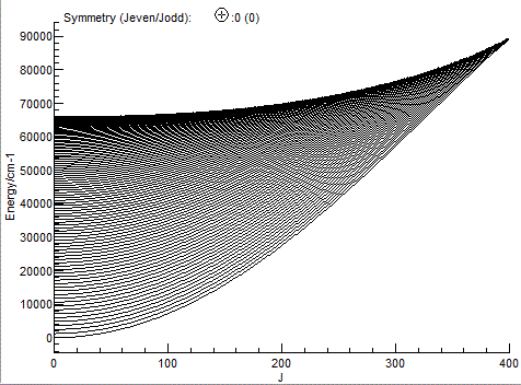
As an example, the ExoMol SiO linelist (http://www.exomol.com/data/molecules/SiO) can be imported directly. At the time of writing, three files are available on the website for the main isotope, 2816for.states, 2816for.trans and 28Si16O-q.txt (the partition function) and these can be imported as is using the procedure above. Importing just the .states file allows an energy level plot to be produced (View, Levels):

With the other two files added general simulations can be produced; the diagram below is at 1000 K assuming a linewidth of 1 cm^-1.

Fitting to the SiO data

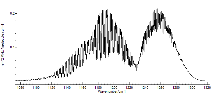
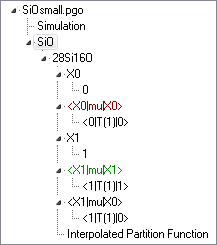
The file SiOsmall.pgo is a standard PGOPHER linear molecule file, set up to simulate the v=0 and 1 levels, and the transitions between them. The partition function is specified numerically by importing the 28Si16O-q.txt mentioned above, so that the line intensities are correct at higher temperatures. The constants were determined by fitting to the ExoMol energy levels. To determine the rotational constants (Origin, B D and H) the following .states file was used as input:

Select J" < 100
StateCols 1
           1     0.000000      1       0    0
           2     1.448467      3       1    0
           3     4.345384      5       2    0
... 800 lines omitted

This is the .states file as above, with the lines referring to the higher vibrational states removed. Note the use of two directives; the Select J" < 100 is one of the standard ones, and is used here to limit the J range of the levels included in the fit as higher J values fit poorly to the standard centrifugal distortion expression. The StateCols 1directive is one described above, and indicates that all the additional quantum numbers are used to provide the state name. For this to work, the vibrational states have to be named "0" and "1".

To determine the three transition dipole moments (0-0, 1-1 and 1-0) the following small .trans file was used as input:

AddStates 2816small.states
Select J" < 10
StateCols 1
Include 2816small.trans

This file includes two other files - note the use of the AddState directive to specify the states; the file 2816small.states is the file used for the energy level fit above. The 2816small.trans file is directly from the ExoMol database; lines not involved in the included .states file are discarded. The other two directives are as above; J is limited to 10 here as the J dependence of the dipole moment is not modelled.