3. General Theory
This general theory chapter is divided into three parts. The first part focuses on a theoretical description of the laser ablation process and is based mainly on thermodynamic and gas dynamic concepts. This is followed by some discussion of the studied materials (Diamond Like Carbon (DLC) and Zinc Oxide (ZnO)). The final section provides an introduction to the theoretical description of periodic solid state structures by ab initio methods, focusing particularly on the bulk crystal and the surface structure of ZnO.
3.1. Laser Ablation
Laser ablation is a macroscopic process, which is difficult to approximate theoretically, mainly because of the extreme conditions that are typically involved. The high photon flux provides essentially instantaneous heating of the material, sometimes to temperatures near the critical point. The material reacts to this temperature increase by evaporation. The particles in the dense emitted gas cloud can also interact with the laser photons, which heats the gas cloud rapidly so that it becomes a plasma. This plasma cloud obtains a high kinetic energy and a high degree of ionisation in this process, which can have interesting implications for material deposition.
3.1.1. Laser interaction with solid material, and particle ejection
The interaction of a pulse of laser light with a solid material can be divided into two sub-categories, depending on the pulse duration. The difference between the two regimes can be explained as follows: laser-solid interactions with nanosecond or longer laser pulses are of sufficient duration to couple not only into the electronic, but also the vibrational wavefunction of the material (phonon relaxation times are typically ~1~5 ps), while for femto/picosecond pulses the duration of the excitation is too short to couple directly into the vibrational wavefunction. Thus laser interactions with these different pulse durations can be expected to induce different ablation behaviours.
3.1.1.1. Nanosecond ablation
The discussion of nanosecond pulsed laser interaction with materials will focus on the ablation of crystalline solids. Polymer ablation is specifically excluded since their excitation with excimer (UV) lasers exhibits a clearly distinguishable photochemical component[1], which is attributable to the unique structure of polymers. The nanosecond ablation of crystalline solids shows very different behaviour and will be discussed in the following paragraphs.
At low fluences, typically around the laser ablation threshold, many of the crystalline solids show a non-thermal particle ejection behaviour when irradiated with visible and especially UV laser pulses. This has been observed in the case of Nd:YAG laser irradiation (at 266, 355 and even 532 nm) of metals [2] and KrF (248 nm) irradiation of graphite [3] and ZnO [4]. The electronic excitation mechanism results in the ejection of high kinetic energy species, which can not be explained by thermal evaporation. This behaviour is normally attributed either to excitation of surface plasmons or to (multiphoton) excitation of surface defects. At higher fluences, any such non-thermal effects decline in relative importance as the thermal evaporation starts to be the dominant mechanism for particle ejection.
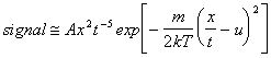
At the typical fluences reported in this thesis (5-20 J/cm2) it is assumed that thermal conduction into the solid and consequent thermal evaporation is the predominant ejection mechanism.[5],[6] The equation governing this thermal ejection mechanism is the well known heat conduction equation:
|
|
where r is the density of the material, Cp is the heat capacity, T is the temperature, t is the time, z is the depth within the material, k is the heat conductivity, R is the material reflectivity, a is the absorption coefficient of the material and I is the intensity of the laser irradiation. It is important to note that the absorption coefficient is actually the only wavelength dependent term in equation (3.1). The absorption coefficient for most known materials rises with increasing photon energy, which explains the preferential usage of UV-lasers for ablation. A high photon absorption coefficient equates to a smaller laser-material interaction region (recall the exponential term in equation (3.1)) and thus to a more efficient coupling of the laser light into the surface region of the target. As a direct consequence laser excitation with longer laser wavelengths yields a higher heat conduction into the bulk of the material, which is an energy loss process in competition with ablation.
This equation can be easily solved for different materials with a finite element calculation, and a number of studies have reported results obtained via finite element calculations for studying the laser melting process of graphite [7] and silicon.[8] The results obtained are in excellent agreement with the experimental data. Material ejection in such cases can be described in terms of thermally activated surface vaporisation, the rate of which is governed by the surface temperature Ts (equation (3.2):
|
|
(3.2) |
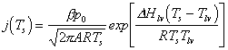
where b is related to the sticking coefficient for surface atoms with atomic mass A. R is the gas constant and the terms Hlv and Tlv are, respectively, the enthalpy and temperature of the liquid-vapour phase transition at an ambient pressure of p0.
The material ejection mechanism and the total amount of flux ejected changes drastically when the fluence increases sufficiently to induce a process called phase explosion, or explosive boiling in the solid material. 6,[9] The phase explosion process occurs in solid targets at temperatures near to the thermodynamical critical temperature of the material, and can be described as a boiling induced by formation of homogeneous nucleation centres at a sufficiently high rate. The laser-induced melt relaxes explosively into a coexistent mixture of liquid droplets and vapour.
The nanosecond ablation of non-polymeric solids can be divided into three regimes, a low fluence regime that is correlated with non-thermal particle ejection, a higher fluence regime (normal deposition fluences) where the laser-material interaction and the particle ejection are well described by a predominantly thermal mechanism and a high fluence limit where the solid reaches its critical temperature and undergoes phase explosion.
3.1.1.2. Femtosecond Ablation
The main model for explaining short laser pulse (< 1 ps) interaction with materials is the two temperature model developed by Anisimov et al.[10] This model describes the temperature dynamics of the material irradiated by an ultra-short laser pulse. The model treats temperature conduction for the lattice and the electrons separately, as shown in equation (3.3). These two equations are coupled by a term that depends on the temperature difference between the two separate systems and an interaction constant, which reflects the strength of the electron-phonon coupling. It is important to note that, over short time scales, the source term (the laser light) appears only in the electron heat conduction equation.
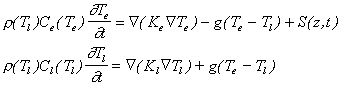
r, C and K and T are respectively the density of the lattice, the heat capacities, the heat conductivities and the temperatures for the two subsystems (the electrons (given by subscript e) and the lattice (given by subscript l)), g is the coupling constant and S is the laser source term.
In this model the laser light specifically heats up the electron distribution. At short time-scales (typically < 1ps), only the electrons equilibrate, via electron-electron coupling, giving an immediate rise in the electron temperature, while the lattice remains at a low (ambient) temperature. The hot electrons start to diffuse within the target material because of the electron temperature gradient. The temperature of the lattice rises over a longer time-scale, which depends on the electron-phonon coupling strength (typical values over the range of 1-5 ps). After this time the electron and the lattice temperatures equilibrate and the system is governed by the standard heat equation. A schematic showing the processes on different time-scales is given in Figure 3.1.
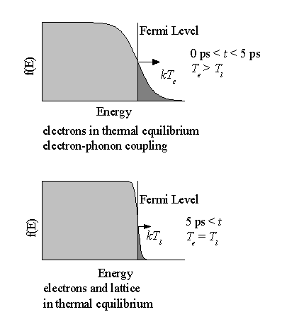
Figure 3.1: Schematic of the processes and regimes in the Two-Temperature Model and the influence on the Fermi-Dirac distribution.
This model has been used extensively to explain melting thresholds for metals;[11]-[13] and the results of such modelling show excellent agreement with experiment. The melting behaviour of semiconductors [14] and graphite [15] under short, intense laser pulse irradiation has also been subject to a number of experimental studies, but these all indicate that melting behaviour in these systems occurs much faster than the typical time-scale implied by the two-temperature model.
For silicon 14, the ultra fast transition between an ordered and disordered phase was studied by means of femtosecond time resolved measurements of the optical reflectivity and the second order optical susceptibility following irradiation with 60-100 fs titanium-sapphire laser pulses. The observed changes in optical properties are consistent with a two-step model involving an initial excitation stage and a subsequent transition stage. The optical properties during the excitation stage are determined by the strong electronic excitation within the material, in particular, by the properties of a dense electron-hole plasma, while the optical properties of the transition stage are governed by the transformation of the crystalline solid to a metallic liquid, illustrated by an observed increase in the reflectivity. The time scale of the entire transformation is measured to be ~300 fs.
For graphite 15, the short time scale laser heating process was studied by measuring the reflectivity of the target under 90 fs titanium-sapphire laser-radiation pulses. As in the case of silicon, an ultra-fast increase in reflectivity was observed. Again this transition to a more reflecting state is interpreted in terms of a transformation from the solid to a liquid metallic phase. The time-scale for the transition in graphite is estimated at ~ 90 fs, even shorter than in silicon.
The theoretical background for this process has been extensively studied by Silvestrelli et al. for both carbon [16] and silicon [17],[18]. These studies show that a very fast disordering of the lattice in these materials can occur at an ionic temperature considerably lower than the melting temperature of the lattice. The laser source term couples directly into the electronic distribution, promoting the electrons into highly excited states. Given this high level of electron excitation the effective ion-ion interactions can change drastically. At high fluences, a large fraction of the electrons are promoted into antibonding orbitals in both materials. The covalent bonds are weakened and the interatomic forces changed by this process. The system responds to the local differences in bonding interaction by ‘melting’ without any appreciable energy transfer between the excited ions and the lattice. This process has been termed ‘plasma annealing’ [19] and can explain the fast transfer from the solid state into an electron-hole plasma. The time-scales of this disordering are calculated to be of the order of 90 fs for graphite and 200 fs for silicon.
The non-thermal nature of the ablation process on these short time-scales also has important consequences for the properties of the ablation plume. The ionic fraction in the ablation plume has been studied for the case of both graphite [20] and titanium [21] targets at a laser wavelength of ~ 800 nm and a pulse duration of ~100 fs by Time Of Flight (TOF) mass spectrometry. An example of the velocity distributions so derived is given in Figure 3.2. Double peak behaviour is clearly evident in this velocity distribution. The slower peak corresponds to a thermal cation distribution with a mean velocity of ~ 60 km/s, while the fast suprathermal peak travels with a velocity of ~ 240 km/s. Such plume splitting behaviour is explicable within the framework of the two-temperature model. Since the electron distribution heats up, the hot electrons are free to escape to vacuum, while the cations remain relatively cold and stationary. Given the high electron density, the Debye length is of the order of a few Angstroms. Thus the cations do not feel the effect of the evolving electric field until the plasma expands and its density decreases to the extent that the Debye length becomes comparable to the plasma dimensions. Once the cations are subjected to the electric field, a fraction of them will accelerate to high velocities. This effect is charge dependent, so it is to be expected that more highly charged particles accelerate to higher velocities and are concentrated in the faster part of the suprathermal peak.
 Figure 3.2:
Velocity distribution of the ions, measured by a Time of Flight ion probe,
arising from laser ablation of graphite at 800 nm using 100 fs laser pulses
Figure 3.2:
Velocity distribution of the ions, measured by a Time of Flight ion probe,
arising from laser ablation of graphite at 800 nm using 100 fs laser pulses
(Qian et al. 20).
3.1.2. Gas and plasma dynamics
At low fluences (i.e. near ablation threshold behaviour), the ejected particles undergo few substantial amount of collisions and their propagation through the vacuum can be approximated as a free flight. However, once more than about one atomic layer is ablated per laser shot this assumption ceases to be valid and gas dynamical effects start to play a significant role in the propagation of the ablation plume.[22]
The gas dynamical equations can be written in the following forms, with the equations expressing the conservation of mass, momentum and energy:
|
|
(3.4) |
|
|
(3.5) |
|
|
(3.6) |
where rv, rve, v, p, av and erad denote the density, internal energy density, hydrodynamic velocity, pressure, the light absorption coefficient of the vapour and the radiative energy losses, respectively. These equations have to be completed by the equation of state relating the pressure to density and energy, namely the ideal gas law:
|
|
(3.7) |
where h is the degree of ionisation and m is the mass of the ablated particles. The internal energy depends on the temperature and the degree of ionisation. This latter quantity can be calculated using the Saha-Eggert equation, which assumes that the plasma is in Local Thermal Equilibrium (LTE).
For nanosecond ablation pulses at the fluence values used in this study, absorption of laser light by the ablation plume is a very significant process, indeed laser plume interaction is often the effect responsible for formation of the ablation plasma. The two main absorption mechanisms in a monoatomic ablation plume are multi-photon ionisation (MPI) and electron-ion inverse Bremsstrahlung (IBE). Electron-neutral inverse Bremsstrahlung is considered to play a minor role under these experimental conditions.5,[23] The absorption coefficients of the two monoatomic processes are given in equations (3.8) and (3.9) for IBE and MPI, respectively;
|
|
where Z is the average ionic state, ni is the concentration of the ions, l is the wavelength of the laser radiation, Te is the electron temperature, Ak is the absorption cross section for a given electronic state k, nk is the concentration of the species in the electronic state (k) to be excited, I is the intensity of the laser and b is the number of photons necessary to ionise the atom/ion. The summation ranges over all the electronic states of the atom or ion to be ionised.
Both of the mechanisms are wavelength dependent. The probability of IBE scales with the wavelength, while MPI scales with the inverse of the wavelength. Thus the importance of IBE increases at longer wavelengths while that of MPI declines. At the wavelengths (193 and 248 nm) used in the present work, MPI is the more important mechanism in ablation plasma formation, although MPI might also serve as a seeding mechanism for IBE. The inverse Bremsstrahlung is highly dependent on the ion (and thus the electron) concentration in the plasma, so its importance can increase during the ablation process.
These absorption processes by the plume not only heat up the plume, but also increase the ionisation fraction and the electron density, thus forming a progressively more dense plasma. At high fluences, the electron velocity distribution that develops from laser plasma heating is no longer described by LTE concepts. Instead of a single Maxwellian distribution, a separate thermal and a hot component with different temperatures can briefly co-exist. This simultaneous existence of hot and thermal electrons in the coronal region of the plasma results in sufficient charge separation to cause strong acceleration of the positive ions in the plasma. The physical mechanisms leading to creation of these fast electrons and ions include resonant absorption of the laser photons and magnetic field effects. In the case of pico/femtosecond laser ablation, the laser-plume interaction is non-existent, since most of the plume development occurs after cessation of the laser pulse.
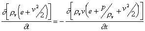
A second approach to describing the plume dynamics follows from theoretical hydrodynamical modelling of the rapid surface vaporisation process associated with the laser ablation process. A rigorous analysis of the process is given in reference [24] and involves the theoretical concept of a Knudsen layer, which defines a collisional regime just in front of the target surface. It has been argued that just 2-3 collisions per emitted particle suffices for formation of a Knudsen layer. The velocity distribution that results when a Knudsen layer forms is given by:
|
|
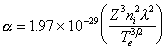
where EI indicates the internal energy of the system, vx, vy and vz indicate the velocity in the three spatial coordinates of a mass m, k is the Boltzmann constant and TK is the temperature of the Knudsen layer. The variable uK is a centre of mass flow velocity in the direction normal to the target surface (x-direction). The flow velocity is related to the surface temperature (Ts) via:
|
|
(3.11) |
Care has to be taken when using such Centre-of-Mass Maxwell Boltzmann (COM-MB) distributions to fit experimental TOF transients, since equation (3.10) is dependent on the velocity (vx,vy,vz) while a TOF transient depends on the position (x,y,z) of the detector relative to the source. The transformation of equation (3.10) into a Time of Flight (TOF) situation is performed by introducing the following simplifying conditions:
· The laser spot size and the detector size are small with respect to their spacing
· The detector is an on-axis detector
· The ejection time (= laser pulse duration) is much smaller than the flight time
Let the detector be located at a distance x normal to the target surface and let the flux of the emitted particles in the range (vx,dvx;vy,dvy;vz,dvz) equate dvxdvydvz ´ vx f(v). Then if y and z are directions parallel to the target surface and t is the flight time then dvy = dy/t, which is expected for a signal that scales with the detector size (dy,dz) and the density (~1/t). Since x is parallel to the target normal and the experiment involves TOF we have:
|
|
(3.12) |
Such is to be expected for a signal that scales as the amount of material into the detector during a temporal window (~x dt/t) and with the density (~1/t). For a flux sensitive detector such as a Faraday Cup, the signal equates:
|
|
(3.13) |
For a density sensitive detector (for example, a mass spectrometer where ions are formed by electron bombardment in the ionisation region) this equation has to be divided by v to yield a t-4 dependence in the pre-exponential factor.
This velocity distribution will be used in Chapter 4 to fit the velocity distributions obtained for the carbon ion signal arising in the 193 nm ablation of graphite. These ion signals were found to be very well approximated by a COM-MB velocity distribution, though the obtained temperatures for these ion distributions are not related to the surface temperature since the ion distribution is subjected to additional heating as a result of laser-plume interactions.
3.1.3. Material deposition
The aspect of material deposition is discussed in detail in Chapter 1.
3.2. Structure of the deposited materials
3.2.1. Diamond Like Carbon (DLC)
DLC is the generic name for carbon-based materials which have a structure and properties that lie between graphite and diamond (the crystalline structures of which are shown in Figure 3.3). DLC materials generally do not possess any long-range crystalline order and contain between 0-60 % hydrogen depending on their formation route. The sp3/sp2 carbon fraction in DLC is also highly dependent on the deposition conditions, and their microstructure is often described as an ensemble of diamond nodules surrounded by a non-diamond amorphous carbon network. The quality of the films is often described in terms of this sp3 to sp2 ratio. The structure of any DLC film is inherently metastable; annealing at high temperatures or with high-energy photons/particles will transform its structure into graphitic carbon.
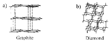
Figure 3.3: Structure of (a) graphite and (b) diamond.
Since it is possible to adjust the sp3 to sp2 content of DLC films by changing the growth conditions, it is possible to tune the optical band gap of the material to a chosen value. Some of these films also show excellent electron emission properties, as a result of their very low or even negative electron affinity (NEA) (i.e. the conduction band is above the vacuum level). This means that the electron emission from the surface occurs readily at relatively low applied potential. This property makes it a candidate for future Field Emission devices (FED’s).
3.2.2. ZnO
ZnO has a tetrahedral coordination; the most common crystal structure at ambient atmosphere and room temperature is the wurtzite structure, shown in Figure 3.4. Another stable crystal structure at ambient conditions is the zinc blende structure, although the lattice energy is slightly higher for this crystal structure.[25] A third possible crystal structure, which is stable at higher pressures, is the rocksalt structure.
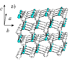
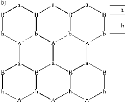
Figure 3.4: (a) Ball and stick image of the wurtzite structure of ZnO, the small balls depict the oxygen atoms, while the larger balls depict the Zn atoms. (b) Picture explaining the stacking sequence along the c-axis, the capital letters stand for Zn atoms.
The experimentally derived values for the a and the c unit cell distances are 3.243 and 5.195 Å, respectively. An important feature of ZnO films deposited by laser ablation methods is that the preferred lattice growth surface is the (002) surface. This is the orientation shown in Figure 3.4, in which the (002) surface is perpendicular to the c-axis. This gives an AbBaAb stacking sequence where capital letters stand for Zn for example and the letter coding is given in Figure 3.4(b). The bulk interplanar distances a and b in Figure 3.4(b) are equal to 0.61 and 1.99 Å.
Zinc oxide is a semi-conductor with a band gap of ~3.4 eV, and a tendency to have a metal excess (i.e. Zn1+xO), which causes it to be an n‑type semiconductor. The excess could be due either to zinc interstitials or to oxygen vacancies.[26]
3.3. Ab initio Theory
3.3.1. The Schrodinger equation and the Born-Oppenheimer approximation
In quantum mechanics, the properties of a system are solely dependent on the wavefunction of the system.[27] The wavefunction is a time and coordinate dependent function, as given in equation (3.14):
|
|
The time dependent part of the wavefunction, the exponential factor, is not dependent on any of the spatial coordinates, while the pre-exponential, spatial coordinate dependent, factor is time independent. Since the two factors in (3.14) are mutually independent it is possible to split the wavefunction into a time-dependent and a time-independent part. Since most of the ab initio theory involves calculation of stationary, time independent, properties we only consider treatments of the time independent wavefunction in this section. The wavefunction is an abstract concept although the square of the modulus of the wavefunction (or, the product of the wavefunction and its complex conjugate) yields the probability that a particle described by the wavefunction is at a certain position in space, thus:
|
|
(3.15) |
which is a statement of the condition that the wavefunction Y is normalised.
As already stated, all the properties of a quantum mechanical system can be calculated from its wavefunction. The most important property of a system is the energy, which can be calculated from the wavefunction using the (time independent) Schrödinger equation (3.16):
|
|
where E stands for the energy of a system described by Y(x,y,z) and ![]() is the Hamiltonian
operator. As can be observed from equation (3.16), solving the Schrödinger equation is in fact an
eigenvalue problem, where Y(x,y,z)
is the eigenfunction of the Hamiltonian operator yielding an eigenvalue E, which is the energy of the system
described by Y(x,y,z). In fact, any (physical) observable can be
represented by an operator of which Y(x,y,z)
is an eigenfunction and the eigenvalues of the operator are the allowed values
of the observable.[28] The non-relativistic Hamiltonian operator
can be written in terms of TN
(the nuclear kinetic energy operator), Te
(the electronic kinetic energy operator) and V (the electrostatic potential energy).
is the Hamiltonian
operator. As can be observed from equation (3.16), solving the Schrödinger equation is in fact an
eigenvalue problem, where Y(x,y,z)
is the eigenfunction of the Hamiltonian operator yielding an eigenvalue E, which is the energy of the system
described by Y(x,y,z). In fact, any (physical) observable can be
represented by an operator of which Y(x,y,z)
is an eigenfunction and the eigenvalues of the operator are the allowed values
of the observable.[28] The non-relativistic Hamiltonian operator
can be written in terms of TN
(the nuclear kinetic energy operator), Te
(the electronic kinetic energy operator) and V (the electrostatic potential energy).
|
|
where R represents the coordinates of the nuclei and r the coordinates of the electrons. The potential energy term in equation (3.17) contains the following components:
|
|
Reflecting, respectively, nuclear-nuclear interactions, electron-nuclear attractions and electron-electron repulsions. The kinetic energy terms in the Hamiltonian (equation (3.17)) can be separated into a term that depends on the electronic coordinates and a term dependent on the nuclear coordinates. The potential energy terms can also be divided into electronic and nuclear dependent parts by making the following approximation: The electrostatic forces felt by the nuclei and the electrons are of similar sizes. Since the nuclei are much heavier than the electrons, the electronic and nuclear motions can be decoupled by assuming that the motion of the electrons can be treated as if the positions of the nuclei are fixed. This approximation is known as the Born-Oppenheimer approximation. Given this assumption, the total wavefunction can be defined using the Born-Oppenheimer product function:
|
|
(3.19) |
where r stands for the electronic coordinates and R stands for the nuclear coordinates. The coordinates in round brackets stand for a variable of the system, while the coordinates in square brackets stands for a parameter of the system. In the same way the potential energy of the system given in equation (3.18) partitions as follows:
|
|
(3.20) |
and can be split into a nuclear and an electronic part. If we neglect the kinetic energy of the nuclei we obtain the electrostatic Hamiltonian, which can be used to solve the electronic wavefunctions at a fixed value of internuclear separation (R).
|
|
(3.21) |
Since electrons are fermions, the wavefunction has to obey the Pauli Principle, which states that the wavefunction has to be anti-symmetric to the exchange of two electrons, or:
|
|
(3.22) |
This also ensures that two electrons, provided they have the same spin, cannot be in exactly the same position:
|
|
(3.23) |
To ensure anti-symmetry, the wavefunction for N electrons can be written as a Slater determinant:
|
|
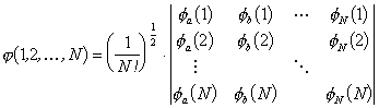
where f is the spin orbital for each electron (the spin orbital contains the spatial and the spin variables). The electron spin is a purely quantum mechanical property (it has no equivalent in classical mechanics) and can take two different values +½ and ½ (often referred to as spin ‘up’ and spin ‘down’).
Exact solution of the electronic Schrödinger equation is impossible, except for simple one-electron systems like H, He+ and H2+. This is the same as stating that the wavefunction and the spin orbitals defined by equation (3.24) are only known exactly for these one-electron systems. For bigger systems the wavefunction has to be approximated in the following way:
|
|
(3.25) |
where gm represents atomic orbitals and ci,m is the contribution each atomic orbital makes to a specific molecular orbital (MO). The wavefunction is thus represented by a Linear Combination of Atomic Orbitals (LCAO). The atomic orbitals for these systems are approximated by 'hydrogen-like' orbitals (i.e. s, p, d etc. orbitals), which have the same angular behaviour as hydrogen orbitals but have an atom dependent radial behaviour. These orbitals are commonly called Slater orbitals. The Slater s-orbitals are difficult to treat computationally (they exhibit a cusp at the origin) and are thus commonly replaced by a combination of Gaussian basis functions (primitives). The assembly of basis functions for a specific atom is called a basis set.
Since the wavefunction for multi-electron systems is not the exact wavefunction of the system, solving the Schrödinger equation for such systems yields an eigenvalue which is similarly an approximation of the exact energy. It can be shown that the eigenvalues obtained with an approximate wavefunction will always be higher than the ground state energy calculated with the true wavefunction. This is expressed mathematically by equation (3.26) for a normalised wavefunction, and is called the variational theorem:
|
|
A consequence of the variational theorem is that the energy calculated with basis sets which are increasingly better approximations of the real wavefunction will yield increasingly lower energies.
During the development of quantum mechanics a large number of schemes were constructed to solve the Schrödinger equation numerically. These methods are called ab initio methods. Such calculations treat a molecule as a collection of positive nuclei and negative electrons that are subjected to Coulombic interactions.
In this study two different types of ab initio calculation were performed, namely Hartree-Fock (HF) and Density Functional Theory (DFT) calculations. Both techniques are discussed in more detail in the following sections.
3.3.2. HF Theory
In HF theory, the Schrödinger equation is solved numerically by the introduction of Self Consistent Fields (SCF). The assumption behind the technique is that any electron moves in a potential which is a spherical average of the potential due to all the other electrons. The Schrödinger equation is calculated for this specific electron in this specific electric field. Since the wavefunction, and subsequently the molecular orbitals for each electron, is not known in advance the final solution of a SCF problem is reached iteratively. First, an initial guess for the wavefunction is provided. With this initial guess, the Schrödinger equation for the individual electrons is solved. The wavefunction so obtained will give an improved averaged potential experienced by the individual electrons, which is used to refine the solution of the Schrödinger equation. This iteration cycle is repeated until the energy change for the system drops beneath a given threshold. This gives a set of self-consistent orbitals.
The Restricted HF theory approximates the structure of a (open or closed shell) molecule as a single Slater determinant (equation (3.24)). The Hamiltonian for this system has the following form:
|
|
(3.27) |
where ![]() is the
'hydrogen-like' Hamiltonian for electron i
in the field of the bare nuclei and the second term in the equation stands for
the electron-electron repulsion (in atomic units). The factor ½ in the electron-electron repulsion is there to avoid
double-counting of the interactions in the double sum.
is the
'hydrogen-like' Hamiltonian for electron i
in the field of the bare nuclei and the second term in the equation stands for
the electron-electron repulsion (in atomic units). The factor ½ in the electron-electron repulsion is there to avoid
double-counting of the interactions in the double sum.
The Hartree-Fock equation for a space orbital ys occupied by electron i in the determinant is:
|
|
where Jr (Coulomb operator) and Kr (Exchange operator) are defined as follows:
|
|
(3.29) |
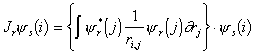
|
|
(3.30) |
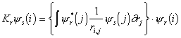
The Coulomb operator takes into account the Coulombic
potential energy of electron i when
its spatial position is given by ys(i)
and when it is interacting with an electron in the space orbital yr.
The exchange term is a quantum mechanical correction term that allows
for the effects of spin correlation.
The sum on the left of equation (3.28) runs over all occupied space orbitals, and the value es is called the one electron orbital
energy. The one electron orbital
energies of the system can be calculated by multiplying both sides of equation (3.28) by ![]() and then integrating
over all space. The total electronic
energy of the molecule is then calculated as:
and then integrating
over all space. The total electronic
energy of the molecule is then calculated as:
|
|
(3.31) |
where Jrs and Krs are the Coulomb and the exchange integrals, respectively.
HF theory provides a first approximation to the wavefunction. Although the theory treats the Pauli exclusion principle correctly, by not allowing two electrons to occupy the same spin orbital, and includes electron-electron repulsion effects in an averaged way, it does not include any direct electron interaction between two electrons of opposite spin. The energy corresponding to this interaction is the energy difference between the true energy of the system and the HF limit and is called the correlation energy. In the following section we discuss a technique that allows calculation of (part of) the correlation energy, namely DFT theory.
3.3.3. DFT Theory
DFT theory adopts a different approach to solving the Schrödinger equation.[29] The basis of the theory is the proof by Hohenberg and Kohn that the ground-state electronic energy is determined completely by the electron density r. The importance of this proof is that the complexity of the wave function will increase upon increasing the number of electrons (the wavefunction is dependent on the coordinates of all the electrons), while the complexity of the electron density is independent on the number of electrons. The main problem of the technique is that each different density yields a different ground-state energy and the functional connecting the energy with the electron density is not known.
As with the HF approach the electronic energy functional may be divided into three parts, the kinetic energy T[r], electron-nuclear attraction Vne[r] and electron-electron repulsion Vee[r]. The electron-electron repulsion can be divided into the Coulomb (J[r]) and Exchange (K[r]) parts and implicitly includes electron correlation in all terms (as opposed to HF theory). The Vne[r] and the J[r] terms are given by their classical expressions.
|
|
(3.32) |
|
|
(3.33) |
Early attempts at deriving functionals for the kinetic and the exchange energy were based on the solution of the problem of a non-interacting uniform electron gas, but this assumption does not hold for atomic and molecular systems, since it fails to predict any bonding between atoms.
The foundations for using DFT in computational chemistry stem from introduction of orbitals by Kohn and Sham.[30] The basic idea of the Kohn-Sham (KS) formalism is to split the kinetic energy functional into two parts, one which can be calculated exactly, the other a small correction term.
Assume a Hamiltonian operator with the following functional form (0 £ l £ 1):
|
|
The ![]() operator is equal to
operator is equal to ![]() for l = 1. For
intermediate l values, however, the
external potential
for l = 1. For
intermediate l values, however, the
external potential ![]() is adjusted so that
the same density is obtained for both l
= 1, the real system, and l
= 0, a hypothetical system with non-interacting electrons. For the l
= 0 case the exact solution to the Schrödinger equation is given as a Slater
determinant composed of MO's, fi,
for which the exact kinetic energy is given by:
is adjusted so that
the same density is obtained for both l
= 1, the real system, and l
= 0, a hypothetical system with non-interacting electrons. For the l
= 0 case the exact solution to the Schrödinger equation is given as a Slater
determinant composed of MO's, fi,
for which the exact kinetic energy is given by:
|
|
The subscript in TS denotes that the kinetic energy is calculated from a Slater determinant. The kinetic energy in equation (3.35) corresponds to the kinetic energy for a system with non-interacting electrons, and therefore equation (3.35) is only an approximation to the real kinetic energy, although the difference between the exact kinetic energy and the kinetic energy calculated with non-interacting orbitals is small. A general expression for the total electronic energy calculated by DFT can be given as:
|
|
(3.36) |
and, by equating EDFT to the exact energy an expression of the exchange-correlation term can be obtained and thus defined as:
|
|
The first term in parenthesis can be considered as the kinetic correlation energy while the second term contains both the exchange and correlation potential energy.
Computationally, the DFT method thus provides a higher level of theory (since correlation energy is taken into account) at a similar computational cost to that of the HF theory. The major problem with implementing DFT methods is the derivation of suitable formulas for the exchange-correlation term. Assuming that an exact functional is available, the problem reduces to solving the determinant of a set of orthogonal orbitals which minimise the energy via an SCF iterative method. The problem can be expressed as the Kohn-Sham equation, which is similar to the Hartree-Fock equation (equation (3.28)).
|
|
(3.38) |
The Kohn-Sham Hamiltonian can be split into different terms:
|
|
(3.39) |
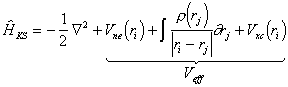
Solution of the Kohn-Sham equation is computationally very similar to solving the HF equation. The numerical methods used for HF theory can also be used for DFT theory and analogously, the KS orbitals can be expanded in a set of basis functions. The advantage of DFT over HF calculations is that the former includes at least an approximation to the correlation energy.
During the development of DFT methods various different functional forms for the exchange-correlation potential have been proposed, spanning a number of different DFT methods. These functional forms are designed to have a limiting behaviour (the uniform electron gas limit) and are determined by fitting parameters to known accurate data. Three different methods have been developed to date; Local Density methods, Gradient Corrected Methods and Hybrid methods.
The Local (Spin) Density Approximation (L(S)DA) assumes that the density is a slowly varying function which can be locally treated as a uniform electron gas. The correlation energy of a uniform electron gas has been determined by Monte Carlo methods for a number of different densities. The results are interpolated using a suitable analytic expression, called the Vosko, Wilk and Nusair (VWN) formula. The L(S)DA approximation generally underestimates the exchange energy by ~10%, thereby creating errors which are larger than the whole correlation energy. Electron correlation is overestimated by a factor of ~2 and, as a consequence, bond strengths are overestimated. Thus notwithstanding the specific inclusion of electron correlation, L(S)DA provides results that are only of a similar accuracy to the HF results.
Improvements to the L(S)DA approach are based on consideration of a non-uniform electron gas. This can be achieved, in part, by making the exchange and the correlation energy depend not only on the density, but also on the derivatives of the density. These so called Gradient Corrected methods involve different expressions for the exchange energy term (ex) and the correlation energy term (ec). Many different functionals have been proposed, each with a specific dependency on the density and its derivatives.
From the Hamiltonian in equation (3.34) and the definition of the exchange energy in (3.37), it is possible to make an exact connection between the exchange-correlation energy and the corresponding potential connecting the non-interacting reference and the actual system. The resulting equation, the Adiabatic Connection Formula (ACF), involves an integration over the parameter l which "switches on" the electron-electron interaction.
|
|
(3.40) |
|
|
|
|
3.3.4. Properties calculated from the wavefunction
As mentioned earlier the wavefunction of a system determines all the properties of that system. The most important property is the energy of the system and the calculation of the total energy via HF or DFT is discussed in the former paragraphs.
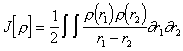
Another important property that can be calculated is the charge distribution in the computed system.[36] This charge distribution determines the bonding behaviour in molecules, and analysis of the charge distribution allows prediction of whether a specific bond is best approximated as covalent or ionic. The charge distribution can be plotted as a charge density plot, or alternatively, a mathematical analysis can be performed, to obtain a more localised picture of the charge distribution. In these charge redistribution schemes, a part of the total electron density is attributed to the atoms contained within the molecule thereby giving a more intuitive picture of the charge localisation. The most widely used scheme for charge redistribution is the Mulliken population analysis.
To illustrate the approach, let us consider the example of a diatomic molecule with one (normalised) atomic orbital on each nucleus, i.e.:
|
|
(3.43) |
If we square the modulus of the wavefunction, integrate and multiply by the number of electrons (N) in the MO, we obtain:
|
|
(3.44) |
where:
|
|
(3.45) |
In the Mulliken population analysis the terms ![]() and
and ![]() are referred to as
the net electron densities on atoms A and B, respectively, and the cross term
are referred to as
the net electron densities on atoms A and B, respectively, and the cross term ![]() is referred to as the
overlap population or the bond order.
If we assume that the cross-term can be divided equally between atoms A
and B, the a gross electron population on each atomic centre can be defined:
is referred to as the
overlap population or the bond order.
If we assume that the cross-term can be divided equally between atoms A
and B, the a gross electron population on each atomic centre can be defined:
|
|
(3.46) |
|
|
(3.47) |
and the gross charge can be defined as the sum of the nuclear and the electronic charge on the atoms. Generalisation of these concepts to extended basis sets and polyatomic molecules is straightforward. It is obvious that this definition contains several arbitrary assumptions. For example, it is highly dependent on the basis set used to describe the system, and the allocation of the overlap distribution to the atoms is arbitrary. Nevertheless, this approach can provide very useful insights into the charge distribution, taking into account the aforementioned restrictions.
3.3.5. Plane Wave Approximation
The system studied theoretically in this thesis (zinc oxide) is a crystalline solid. The approach to calculating the electronic structure and properties of solids is summarised in the Bloch theorem. This assumes that the wavefunctions of the electrons in a crystal have the Bloch form:[37]
|
|
(3.48) |
where uk(r) is a function that has the lattice periodicity,
i.e. uk(r) = uk(r+tm)
where tm is any relative
lattice translation. The Bloch
function, Yk consists
of a free electron wavefunction ![]() , modulated by the uk
function that has the periodicity of the lattice. Thus it is a modulated plane wave. It can be readily proven that the wavefunction must be of the
form
, modulated by the uk
function that has the periodicity of the lattice. Thus it is a modulated plane wave. It can be readily proven that the wavefunction must be of the
form
|
|
(3.49) |
which is the Bloch condition on the wavefunction. In this way the Bloch theorem ensures that the periodicity of the crystal structure is reflected in the periodicity of the electronic structure. This theorem also enables calculation of the electronic structure of a crystal lattice by calculating the wavefunction of the appropriate unit cell. The assumption that the electronic wavefunction is a plane wave in the three dimensions readily extends this solution to the whole crystal lattice. Surfaces can be studied also, by assuming electronic periodicity in only two dimensions, while the electronic structure in the third dimension is calculated independently.
3.3.6. Polar surfaces in solids
Polar surfaces of compound materials are of prominent interest. The orientation of the surface is such that each repeating unit perpendicular to the surface bears a non-zero dipole moment. The resulting macroscopic dipole moment induces an electrostatic instability, which can only be cancelled by the introduction of compensating charges in the outer planes. The various ways by which the lattice can electronically relax are discussed below.[38]
The importance of polar surfaces to the present work follows from the observation that the dominant growth surface of ZnO, the (002) surface, is a polar oxide surface. To understand the implications of this observation we have performed ab initio calculations to assess the electronic structure of this surface. The results are discussed in Chapter 5.
3.3.6.1. Criterion for surface polarity
According to classical electrostatic criteria, the stability of a surface depends on the characteristics of the charge distribution of the repeating structural unit in the direction perpendicular to the surface. Three different cases can be distinguished and are shown in Figure 3.5.[39] Type 1 and 2 surfaces have a dipole moment in their repeat unit and are thus potentially stable. In contrast, type 3 surfaces have a diverging electrostatic surface energy, not only because of the dipole moment on the surface, but also on all of the repeating units throughout the material.
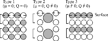
Figure 3.5: Classification of different surfaces. [ Indicates the extent of the repeat unit and circles with different colours represent the different ions in the lattice. Type 1 and type 2 are stable surfaces, the difference between the two being that surface 2 has a non-zero charge separation along the axis normal to the surface (Q ¹ 0). Type 3 surfaces are inherently unstable since they also exhibit a dipole moment along the axis normal to the surface.
A simple representation of the electrostatic field and potential generated by a Type 3 surface along the polar direction is given in Figure 3.6. Two layers with opposite charge ±s alternate along the surface normal, with interlayer spacing R1 and R2. The total dipole moment (M = NsR1) is obviously proportional to the slab thickness in (a), which, in the limiting case of an infinite number of layers, makes the surface energy divergent. To stabilise the surface, the charge density of the most outer layers can be modified so as to cancel out the macroscopic component of the dipole moment and thereby cancel the polarity. This can be achieved by assigning a value given by equation (3.50) to the charge density on the outer layers of the slab, as shown in Figure 3.6(b).
|
|
This results in a total dipole
moment ![]() , which is no longer proportional to the slab thickness.
, which is no longer proportional to the slab thickness.
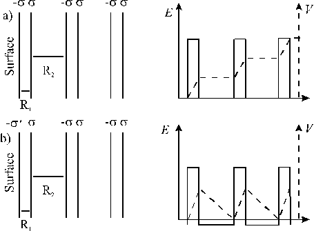
Figure 3.6: Spatial variation of the electrostatic field and potential generated along the polar direction in a type 3 surface, (a) without surface relaxation (yielding surface energy = ¥) and (b) with surface relaxation (yielding a finite value for the surface energy).
A polar surface can thus be stabilised by a charge compensation in the outer layers. This implies that either the charges or the stoichiometry in the surface layers needs to be modified in comparison with their bulk values to achieve polar surface stabilisation. The different scenarios to cancel the polarity are thus:
· Stoichiometry changes in one or several surface layers. This can lead to phenomena like reconstruction and terracing, depending on the order within the vacancies or adatoms.
· Inclusion of foreign atoms or ions, coming from the residual atmosphere in the experimental set-up, to provide the necessary charge compensation.
· Charge compensation may result from an electron redistribution in response to the polar electrostatic field. This can be studied in some detail by ab initio calculations.
Which relaxation mechanism will be the most favourable is dictated by energetic considerations. There will always be enough electronic degrees of freedom to relax the material via the third of the above mechanism, but, in most cases, one of the other two mechanisms will actually provide a route to a lower surface energy.
3.3.6.2. Relevant processes for cancelling the polarity
The mechanisms that govern electron redistribution within the lattice, and thus the polarity of the lattice, are now discussed in more detail.
One process that can be considered is surface relaxation. As Figure 3.6 shows, surface relaxation will not cancel the polarity if the relaxation is not accompanied by a change in the surface layer charge densities, since the dipole moment is determined by the charges and layer spacings in the bulk unit. Furthermore surface relaxation will only stabilise an electrostatically stable surface.
Similarly, change in covalency in the surface layers will not contribute much to the stabilisation of these polar surfaces. Again Figure 3.6 readily shows that reduction of the charge on the two top layers, because of an increase in covalency, will not cancel the polarity.
Charge compensation on stoichiometric surfaces can only be achieved by a formal charge transfer from one surface to the other surface, thereby creating an 'induced dipole moment' which counteracts the original dipole moment. This is achieved by partially filling the conduction band surface states or by depleting the valence band surface states.
The second way the lattice can relax is via a change of the surface stoichiometry. For example, to remove the charge necessary to counteract the dipole moment on a ZnO (001) surface can be calculated with equation (3.50) and is ~ ¾ of the total charge density (R1=0.61 and R2=1.99 Å). So, to counteract the bulk dipole moment, ¼ of the cations and anions in the ZnO surface layer have to be removed.
3.3.6.3. Former studies on ZnO
The (001) Zn terminated and ![]() O terminated surfaces
of ZnO have been studied by grazing incidence X-Ray diffraction (GIXD).[40] In this study the Zn terminated surface
shows a +0.05 Å outward relaxation associated with a 0.75 occupancy of the Zn
sites in the outer layer. The O
terminated surface is relaxed inward by -0.03 Å, and the occupancies of both
the outer and the underlying layers are different from their bulk value. This picture illustrates that a ZnO polar
surface relaxes preferentially by changing the surface stoichiometry rather
than via charge redistribution.
O terminated surfaces
of ZnO have been studied by grazing incidence X-Ray diffraction (GIXD).[40] In this study the Zn terminated surface
shows a +0.05 Å outward relaxation associated with a 0.75 occupancy of the Zn
sites in the outer layer. The O
terminated surface is relaxed inward by -0.03 Å, and the occupancies of both
the outer and the underlying layers are different from their bulk value. This picture illustrates that a ZnO polar
surface relaxes preferentially by changing the surface stoichiometry rather
than via charge redistribution.
Theoretical LSDA calculations on embedded clusters [41]
have shown that spontaneous charge redistribution takes place on stoichiometric
terminations, as expected from the electrostatic criterion. This has been attributed to a change in
covalent bonding character on the Zn face, and a partial filling of the surface
states on the oxygen face. In a very
recent study [42], the polar
(001) and ![]() surfaces have been
geometry optimised to yield an energy minimum with relatively small
relaxations. The calculations indicate
that the surfaces are stabilised by a charge transfer between the two surfaces
of 0.17 e, which leads to metallic
surface states.
surfaces have been
geometry optimised to yield an energy minimum with relatively small
relaxations. The calculations indicate
that the surfaces are stabilised by a charge transfer between the two surfaces
of 0.17 e, which leads to metallic
surface states.