3. Experimental

 

3.1. Introduction

 

Diamond films were deposited onto silicon (100) single crystal substrates using a microwave plasma assisted CVD reactor.  Deposited films were characterised by SEM (Section 2.2) and LRS (Section 2.3) allowing determination of film morphology, crystallinity and quality.  Most of the films deposited from S containing gas mixtures were also subjected to XPS analysis (Section 2.4) and also four-point probe measurements (Section 2.5) in order to determine film sulfur content and resistivity, respectively.  Details of both the film deposition and analysis experiments are given in the first part of this chapter, while the analysis of the microwave plasmas used for film growth is discussed in the second part.  The techniques used to investigate these plasmas were optical emission spectroscopy and molecular beam mass spectrometry.  Additional mass spectroscopic investigations were also undertaken of hot filament activated H/C/S containing diamond CVD gas mixtures.

 

Growth of films at reduced substrate temperature has been investigated using an input gas mixture of 50%CH₄/50%CO₂, while sulfur doping of films has been attempted using xH₂S/1%CH₄/H₂, xH₂S/51%CH₄/49%CO₂ (x = 0-5000 ppm) and 0.5%CS₂/H₂ feedstock gas mixtures.  Plasma chemistry has been investigated as a function of CH₄/CO₂ ratio (for the first gas mixture) and H₂S addition.  Mass spectroscopic studies were also undertaken in which a hot filament was placed into the MWCVD reaction chamber.  This allowed the effects of H₂S addition to a 1% CH₄/H₂ gas mixture, and hot filament temperature on 0.5%H₂S/1%CH₄/H₂ and 1% CS₂/H₂ gas mixtures, to be studied. The results of both film and gas phase characterisation will be presented together, in the following chapters, for each of the gas mixtures investigated.

 

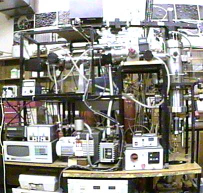
Figure 3.1. Photograph of experimental apparatus used in this work.

 

3.2. Film deposition apparatus

 

The following section describes the microwave plasma CVD (MPCVD) apparatus used to deposit diamond films.  The system components are shown in black in the schematic diagram presented in Figure 3.2.  The molecular beam mass spectrometer system components are also shown (in red and blue), and will be discussed in Section 3.5.

Figure 3.2. Schematic diagram of experimental apparatus (adapted from Reference [1]).

 

3.2.1. Microwave System

 

The microwave generator (ASTeX 1500 W S-1500i) used a magnetron to generate 2.45 GHz microwave radiation that was then directed down a rectangular air filled metallic waveguide.  A circulator allowed the microwave radiation to travel towards the CVD reaction chamber, but redirected any reflected microwaves into a water-cooled dummy load.  In this way any excess energy was dissipated, thus preventing damage to the magnetron.  Two meters were use to monitor the forward, and reflected microwave power.  Reflected microwaves resulted from incorrect tuning of the CVD reactor chamber.  The microwave power applied to the reaction chamber was therefore the forward power minus the reflected power.  A mode converter was used to couple the microwave energy into the reactor via a movable antenna.  A reflective metal blanking plate terminated the waveguide.  The bottom of the mode converter was bolted onto the top of the reaction chamber.  Microwaves could then pass into the chamber, through a quartz window (1 cm thick and diameter of 12 cm).  The window was vacuum-sealed by two Viton O-rings.

 

3.2.2. Deposition Chamber and Vacuum System

 

The main deposition chamber consisted of a double-skinned stainless steel cylinder with an inside diameter of 147 mm.  Water-cooling prevented both damage to, and chemical reactions on, the inside reactor wall.  Two view ports were mounted opposite each other.  These allowed the deposition process to be monitored through 38 mm glass windows mounted in Conflat 75 mm outside diameter flanges.  These glass windows could be removed and replaced with quartz ones during optical emission spectroscopic studies of the microwave plasma.  A loading door was placed at 90° to both windows and allowed wafers of up to 100 mm diameter to be placed into the reactor.  The door was sealed by a Viton O-ring and was held shut by the difference between atmospheric and the reduced pressure maintained within the reactor during deposition.

 

Opposite the loading door was a 100 mm internal diameter port that led to a Conflat 150 mm vacuum flange.  This flange provided a mounting for the sampling probe during MBMS experiments, the probe being absent during film deposition.  The base pressure of the reaction chamber was evaluated using an Edwards PR10-K Pirani vacuum gauge (10^-3-1 Torr), while process pressure was monitored by a Tylan General CDL-21 (0-100 Torr) Baratron during deposition experiments.

 

3.2.3. Cooled Substrate Holder

 

A 100 mm diameter molybdenum substrate holder was mounted axially in the reactor with a bellows at its base allowing vertical translation of the substrate holder and substrate.  Such adjustment of the chamber geometry was necessary in the microwave cavity tuning process to improve the matching of the microwave circuit.  In order to reduce the substrate temperature during deposition runs, the heated substrate holder assembly used in previous work [1] was replaced by a cooled substrate holder.  The development of the substrate cooling system is described below, but the general apparatus will be discussed here.  Water from the mains supply was circulated through a coil of copper pipe situated in a plastic water reservoir (see Figure 3.3).  Water in the reservoir was thus cooled before being pumped through plastic Swagelok tubing, copper piping placed below the molybdenum substrate holder, and back into the reservoir.  The water flow through this closed cooling loop had two settings, full and low.  The required temperature was set on the control box.  A K-type thermocouple, clamped into a recess in the underside of the substrate holder, allowed a Eurotherm 2132 control box to monitor substrate holder temperature and control it by switching between water flow settings. 

 

The use of cooling water flow rates was found to control the substrate temperature within a relatively narrow (~50ºC) temperature range.  In order to attain a wider range of substrate temperatures (~400-870ºC) it was found necessary to fabricate a number of stainless steel spacers, for placement between the cooling pipes and the molybdenum substrate holder.  Four such spacers were manufactured in the form of steel rings, each with outside and inside diameters of 104 mm and 84 mm.  The spacers were 1, 2.5, 5 and 10 mm thick. 

Thus, it was possible for the user to predetermine the substrate temperature by placing suitable spacers between the copper cooling pipes and the molybdenum substrate holder and setting the desired temperature on the cooling system control box.  Details of the calibration procedure allowing the thermocouple reading to be related to the temperature of the growing diamond surface are given in Section 3.2.3.2.

 

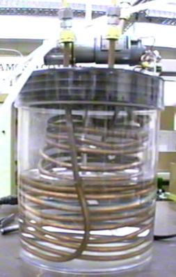
Figure 3.3. Photograph of water reservoir for cooled substrate holder.

 

3.2.3.1. Cooled Substrate Holder Development

 

The first set-up (Figure 3.4) made use of a copper pipe coil, clamped to the underside of the molybdenum substrate holder.  The spring was intended to allow spacers to be placed between the cooling coil and the substrate holder (with access via the reactor chamber door), thus allowing the degree of cooling to be varied.  The substrate holder was electrically isolated from the rest of the apparatus by the use of plastic water pipe connections and glass insulation for the thermocouple.  The tip of the thermocouple was electrically isolated from the molybdenum substrate holder by diamond.  Such electrical isolation of the substrate holder was intended to allow possible future studies of biased enhanced nucleation to be undertaken (Reference [2] and references therein).

 

During the first test of the substrate cooler problems were encountered with secondary plasmas and erratic pressure variations within the chamber.  The thermocouple also failed.  When the apparatus was dismantled it was found that secondary plasmas had formed below the substrate holder causing the plastic water pipe connections to melt.  This had caused water to leak into the chamber, causing the pressure variations observed.  It was also discovered that another secondary plasma had burnt through the thermocouple wire and also destroyed the diamond insulation.

Figure 3.4. Initial design for cooled substrate holder: (a) placement of assembly within reactor chamber, (b) details of substrate holder.

 

A number of modifications were made to the substrate cooler to improve its reliability (Figure 3.5).  A skirt of stainless steel was added to the substrate holder in order to prevent the formation of secondary plasmas below it.  The plastic pipe connections were replaced with steel fittings, and both the thermocouple and thermocouple wires were protected by steel tubing.  The thermocouple was now clamped to the back of the substrate holder by being screwed into the thermocouple protection tubing (Figure 3.6).  This replaced the spring mechanism as it was found that it was impractical to change spacers without removing the substrate holder from the chamber, as originally intended.  A base plate was also added to the chamber to clamp the water-cooling pipes (and therefore the substrate cooling assembly) into a central position.

                           (a)                                                                 (b)

Figure. 3.5.  Modified cooled substrate holder: (a) placement in deposition chamber, (b) detail of substrate holder.

 

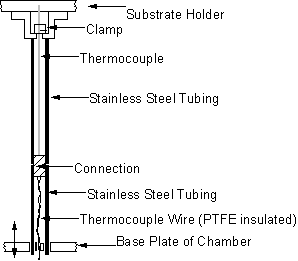
Figure 3.6. Protection of substrate holder thermocouple.

 

3.2.3.2. Calibration of Substrate Temperature Measurement

 

The substrate temperature was monitored via a K type thermocouple (TC1) clamped onto the underside of the substrate holder (~ 3 mm from the surface).  Calibration experiments were performed enabling this thermocouple temperature reading to be scaled to give an accurate value of the true temperature of the substrate surface.  The calibration was performed in two stages, over two different temperature ranges.  For substrate temperatures below 600°C a second K type thermocouple (TC2) was clamped directly onto the surface of a Si substrate sitting on the substrate holder within the reaction chamber.  An electric heater element was then placed above (~5 mm) the substrate and the chamber was evacuated before being filled with a 50% CO₂/50% CH₄ gas mixture at a pressure of 40 Torr (see Figure 3.7). 

 

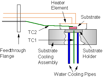
Figure 3.7.  Calibration of substrate temperature measurement at low temperatures (<600°C).

 

Comparison of the true substrate temperature from TC2 with that measured by TC1 allowed TC1 to be calibrated. 

 

Calibration measurements for substrate temperatures above 600°C were carried out during normal deposition runs, using a 2 colour optical pyrometer.  A calibration graph was plotted using the results from the high and low temperature experiments (Figure 3.8) allowing TC1 to be used in all future experiments to give an accurate measure of the true substrate temperature.

 

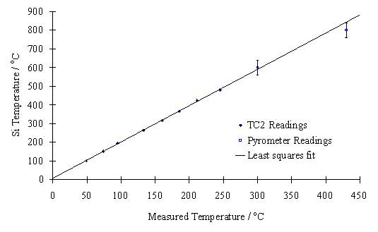
Figure 3.8.  Calibration graph showing Si substrate surface temperature, measured by thermocouple (TC2) and pyrometer, versus temperature measured by TC1.

 

The temperature reading from TC1, T_meas can therefore be converted into the substrate surface temperature, T_sub, via Equation 3.1.

 

                          Equation 3.1

 

As TC1 is clamped directly to the back of the molybdenum substrate holder the distance between it and the substrate surface is not changed by the use of spacers (Section 3.2.3).  Therefore Equation 3.1 is valid regardless of the spacers used.

 

3.2.4. Gas supply

 

Gas supply was via standard gas cylinders (BOC, 2000 psi), lecture bottles (Argo International; Ltd, 1000 psi) or, in the case of CS₂, the vapour pressure (< 1 atm) above a liquid sample contained in a gas bulb.  In all cases brass regulators were used (except CS₂ where no regulator was needed).

 

Regulators were used to reduce the cylinder gas pressure down to ~ 20 psi.  Input gas flows were regulated by the use of mass flow controllers (MFCs) thus allowing control over the input gas mixture.  As Figure 3.9 shows, each gas passed from the cylinder regulator, through a manual shut off valve, MFC and into a manifold where the separate gases were mixed prior to passage through another manual shut off valve, solenoid valve and into the reaction chamber.

 

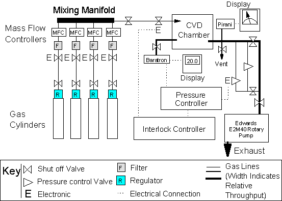
Figure 3.9. Gas supply, pressure control and exhaust system.

 

MFCs are factory calibrated against a test gas, therefore a gas conversion factor (GCF) is required if the MFC is to be used for a gas other than the test gas.  All flow controllers used were of the type FC 260 Viton MFC (Tylan General), with calibration gases and relevant GCFs [[3]] set out in Table 3.1. 

 

Equation 3.2 gives the control box settings for a given flow of a gas through an MFC.  Here the Scale Factor is calculated using the full scale deflection, FSD, of the MFC control box flow gauge and the maximum flow rate for the MFC, by Equation 3.3.

 

               Equation 3.2.

 

                   Equation 3.3.

 

Table 3.1. Table of gas source and MFC details for experimental work.

 

It should be noted that when H₂S dilutions (i.e. 1% in H₂ or CH₄) were used, gas flow was set using the GCF of the dilution gas. 

 

The reaction gas mixture was introduced into the reactor chamber via a ring-shaped ‘sprinkler’ tube incorporated into the topmost flange of the reactor body, positioned just below the quartz window.

 

3.2.5. Pressure Regulation and Exhaust System

 

The lower portion of the deposition chamber contained two ports, one led to the Baratron pressure gauge and the other was an exhaust line.  The exhaust line included a vent valve (used to bring the deposition chamber up to atmospheric pressure) and a Pirani pressure gauge.  The exhaust split into two separate paths, a wide tube (high conductance) and a smaller (low conductance) tube, before rejoining (both tubes having manual shut off valves).  The exhaust line was pumped by an Edwards E2M40 two stage rotary vacuum pump, which achieved a deposition chamber base pressure of ~10^-1 Torr. 

 

When the chamber was evacuated to base pressure, all the exhaust lines were left open to allow maximum conductance of gases to the pump.  In order to control the chamber pressure during deposition, the high conductance line was shut off.  The low conductance line was split into two parallel pipes, one with a manual needle valve and the other an electronic control valve (MKS Type 248 A 10000 CV).  The electronic valve was connected to an automatic pressure controller (Tylan General Model 80-1), which was also connected to the Baratron pressure gauge.  It was therefore possible for the controller to both monitor and control the pressure of the deposition chamber, although problems were encountered regarding the use of CH₄/CO₂ gas mixtures (as described in Section 3.2.10.1).  Such control was possible over the pressure range 1-100 Torr, to within 0.1 Torr.  Gases exiting the pump entered an exhaust line and were thus removed from the building in a safe manner.

 

3.2.6. Substrates: Selection and Preparation

 

Deposition was carried out using single crystal (100) silicon wafers.  Initially n-type substrates were used for investigations restricted to observation of film morphology and quality.  However, it was found that these highly conductive (1-10 W cm) substrates unduly influenced electrical (e.g. four-point probe) measurements of diamond films deposited on them.  Therefore, films intended for such measurements were grown on highly resistive (~10⁵ W cm) undoped Si substrates.  Silicon substrates were broken into rough squares (~ 20 mm²) before being manually abraded with 1-3 mm diamond grit.  This abrasion produces microscopic scratches in the surface of the substrate, which are found to promote diamond nucleation.  Substrates were then cleaned using isopropanol and cotton buds. 

 

Deposition was also attempted using single crystal (100) HPHT grown diamond substrates. These substrates were ~2 mm² ´ 0.5 mm thick, translucent light yellow in colour and were obtained from Ando at NIRIM in Japan.  Substrate preparation involved washing with isopropanol and wiping with cotton buds prior to deposition.

 

3.2.7. Safety Interlock System

 

In order to allow limited unattended operation of the microwave reactor a system of interlocks was present, having three main functions.  Firstly, the chamber cooling water flow rate was measured, and if this dropped below a preset value  the microwave power supply shut off and the solenoid valve in the chamber gas supply line shut.  Secondly, the pressure of the deposition chamber was monitored, and if it strayed more than 1 Torr from the set value the microwave power and gas supply were again shut off.  Such pressure variations result from the plasma jumping to different positions within the reaction chamber.  This interlock is primarily intended to prevent damage to the quartz window from occurring, in the event that the plasma jumped to a position adjacent to it.  Lastly, the temperature of the substrate cooling water was monitored, and if this rose above 60°C the water flow rate was set to full.  If the water rose to a temperature of over 90°C then the microwave power and gas lines shut off.  Thus, if any of these interlocks were tripped the chamber safely pumped down to its base pressure.

 

3.2.8. Deposition Experiment Procedure

 

Results for deposition experiments are given in Chapters 5-7.  Here the operating procedure followed during these investigations will be detailed.  The reaction chamber was normally left evacuated while not in use.  Therefore, all shut off valves situated between the chamber and Edwards pump were closed.  The vent valve was then opened to bring the chamber up to atmosphere.  The loading door was then opened, allowing the substrate to be placed (as described in Section 3.2.9) on the substrate holder.  The loading door was then shut, before the gas lines to the pump were opened, enabling the chamber to be pumped down to base pressure.  All valves in the gas lines between the cylinder manual shut off valves and the reaction chamber were then opened.  This allows the gas lines to be evacuated (usually overnight).

 

To begin a deposition run, the high conductance gas line between the chamber and the rotary pump was then shut off.  The chamber was then filled with 20 Torr of the gas mixture required to strike the plasma controlled by the automatic pressure control valve.  This mixture was either 100%H₂ (in the case of 1%CH₄/H₂ gas mixtures) or ~50%CH₄/50%CO₂.  The substrate cooler control box, microwave power supply and chamber cooling water were then switched on.  The substrate cooler temperature was then set, before the microwave power was applied to the reaction chamber (~200 W).  The reflected microwave power was then minimised by tuning the microwave mode converter.  The microwave power was then slowly increased in 200 W jumps.  Each time the microwave reflected power was, again, minimised.  Once the microwave power reached 1000 W, and the reflected power minimised, the plasma was usually visible in the gap between the substrate holder and the chamber wall.  Increasing the microwave power to ~ 1200 W induced the plasma to jump into a position above the centre of the substrate holder.  The applied microwave power was then reduced to 1000 W and reflected power was again minimised.  The chamber pressure was then increased to 40 Torr.  Once the pressure stabilised, the chamber pressure and cooling water interlocks were activated (Section 3.2.7).  In the case of 50%CH₄/50%CO₂ gas mixtures, this time was then recorded as the run start time.  For sulfur doping experiments, using 51%CH₄/49%CO₂, H₂S was then introduced and the run start time recorded.  Otherwise, in the case of sulfur additions to 1% CH₄/H₂ gas mixtures, 1%CH₄ and H₂S were now introduced, and the run start time recorded.

 

After the required deposition time (usually 8 hours), the interlocks were switched off and microwave power was slowly reduced and shut off.  The chamber was then allowed to cool, either in 20 Torr of CO₂ or H₂, as dictated by the gas mixture in use.  When the substrate cooler controller displayed a temperature reading of <40°C, the cooler and gas flow were shut off.  All gas lines between the chamber and the rotary pump were then opened, allowing the chamber, and gas lines back as far as the cylinder manual shut off valves, to be evacuated.  All valves between the cylinders and the rotary pump were then shut off.  The chamber was then vented to atmosphere, allowing removal of the substrate through the loading door.  The chamber was then left under vacuum by opening all valves between the chamber and rotary pump.

 

 

 

3.2.9. Placement of Substrates during Deposition

 

  The substrate mounting was dependent upon which experiment was being carried out.  For depositions using a 50% CH₄/50% CO₂ gas mixture at various substrate temperatures, the substrate was placed directly onto the centre of the cooled molybdenum substrate holder.  Depositions involving H₂S addition to 1%CH₄/H₂ gas mixtures were carried out with the substrate holder covered using a blank Si wafer, since it has been reported that hot Mo possibly acts as a sink for gas phase S species, scavenging them and reacting to form solid MoS₂ [[4]].  Substrates were placed on an alumina plate on top of this Si cover wafer.  Experiments involving H₂S/51%CH₄/49% CO₂ gas mixtures at high substrate temperature, T_sub, (900°C) also used this substrate mounting.  Lower temperature depositions using this gas mixture were carried out with the substrate placed directly on the Mo substrate holder, thus allowing T_sub to be maintained at 620ºC using a substrate holder cooling system as discussed in Section 3.2.3.  The substrate was surrounded by Si wafer fragments, covering the Mo substrate holder to prevent any possible scavenging of S as discussed above. 

 

These different substrate mounting arrangements led to differing plasma-substrate interactions.  When the substrate is placed directly onto the Mo substrate holder, the separation between it and the plasma is ~ 2 mm.  However when placed on alumina, on top of a Si wafer, the Si wafer often buckled up into the plasma (as a result of plasma heating).  This resulted in the substrate being raised into contact with the plasma, enabling automatic heating of the substrate to ~900°C (measured by a two colour optical pyrometer).  It was therefore possible to deposit films using 1% CH₄/H₂ gas mixtures, at the T_sub required for diamond growth, without replacing the cooled substrate holder with the heated unit used in previous deposition experiments using such mixtures [1].  However, such differences in plasma-substrate interactions (as illustrated in Figure 3.10) must be considered when interpreting the results of deposition experiments.

 

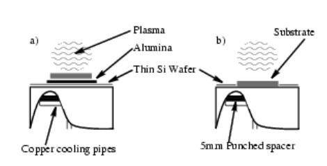
Figure 3.10. Cut-away diagram illustrating plasma-substrate interaction with the substrate positioned (a) on alumina, placed onto a Si cover wafer and (b) directly on the substrate holder, (adapted from Reference [5]).

 

3.2.10. Problems Encountered during Deposition Experiments

 

The use of CH₄/CO₂, and sulfur containing gas mixtures was found to cause problems during CVD film deposition experiments.  These difficulties were not experienced during previous work using 1% CH₄/H₂ gas mixtures [1] in an identical reactor.  Each set of problems is dealt with separately in the following sections.

 

3.2.10.1 CH₄/CO₂Gas Mixtures: Chamber Pressure Control

 

It was discovered that when using CH₄/CO₂ gas mixtures, the electronic pressure control valve failed to control the reactor chamber pressure adequately.  A replacement valve failed to remedy the problem, which was only solved by the addition of a manual control valve.  This was placed in parallel with the electronic valve, and was used to make manual pressure adjustments as and when necessary (approximately every 20 minutes).  The cause of this problem is not clear. 

 

 

 

3.2.10.2 Sulfur Containing Gas Mixtures

 

Use of gas mixtures containing sulfur at concentrations >1000 ppm species (e.g. H₂S/1%CH₄/H₂, H₂S/51%CH₄/49%CO₂ or CS₂/H₂) was observed to result in significant deposition of yellow sulfur powder on the reactor chamber walls.  This necessitated the cleaning of the chamber after deposition, OES and MBMS experiments using such gas mixtures.

 

3.3. Film analytical apparatus

 

This section describes the experimental details of the methods used to analyse deposited films, as introduced in Chapter 2.  Experimental and data processing procedures will be laid out for SEM, LRS, XPS and Four-point probe techniques.

 

3.3.1. Scanning Electron Microscopy

 

Analysis was carried out using two instruments.  Firstly, a Hitachi S-2300 SEM producing images in the form of 35 mm negatives (the prints of which are presented here), and also a JEOL 5600LV SEM producing electronic images in the form of “bit map pictures”.  SEM images for all films analysed are presented in Appendix 2.

 

3.3.2. Laser Raman Spectroscopy

 

Two separate systems were used to analyse films, both of which operated at an excitation wavelength of 514.5 nm.  The first instrument contained a Dilor – XY double spectrometer (see Chapters 5 and 6), while the second utilised a Renishaw 2000 spectrometer (see Chapter 7).  In both cases a plasma filter was needed to filter out emission lines produced by the (Ar⁺) laser system.  Laser light was focused through a ×50 objective lens producing a spot size of ~10 mm on the surface of the sample.  A number of exposures (10–30), each of 1 s duration, were collected during film analysis.

Where utilised, curve fitting of spectra was carried out using the Renishaw WiRE (windows-based Raman Environment) software package.  Gaussian lineshapes and either linear or quadratic baselines were employed.  Fitted curves were then used to estimate the quality of deposited diamond films, both by calculation of the ratio I_d/I_G, and also the quality factor Q, as discussed in Section 2.3.  Raman spectra and curve fits are presented in Appendix 2.

 

3.3.3. X-ray Photoelectron Spectroscopy

 

Diamond films were analysed by a Fisons Instruments VG Escascope in the Bristol Interface Analysis Center, using a Mg K X-ray source (300 W), with a field of view of 700 µm.  Wide scans were collected over an energy range of 0-1000 eV.  Scans over smaller ranges were then carried out for the following peaks: C 1s (164 eV), O 1s (532 eV), S 2p (284 eV).  All XPS spectra obtained are presented in Appendix 3.  The integrated areas of each peak, A_x, and the peak sensitivity factor, S_x, were then used to calculate atomic ratios, R_x, of S relative to C, using Equation 3.4.

 

                                         Equation 3.4

 

Using sensitivity factors for S and C of 0.25  and 0.54,  respectively S/C film content ratios can be established.

 

3.3.4. Four-point Probe Measurements

 

Electrical measurements of S-doped films were made by placing four spring‑loaded (Au) probes, in a linear geometry and with a spacing, s, of 2.5 mm, onto the diamond surface (see Figures 3.11 and 3.12).  Measurements were made with the apparatus placed inside a Faraday cage that provided shielding from any external electric fields.  A fixed electric current was passed through the sample, between the outer two probes, while the voltage across the inner two was recorded.  A Solartron SI 1287 potentiostat instrument carried out both application of current and voltage measurement.  Voltage readings were taken for a range of applied currents, allowing V/I curves to be plotted,  the gradient of which corresponds to the measured film resistance between the inner two probes. 

 

Figure 3.11. Photograph of four-point probe apparatus showing electrical connections, sprung probes and sample.

 

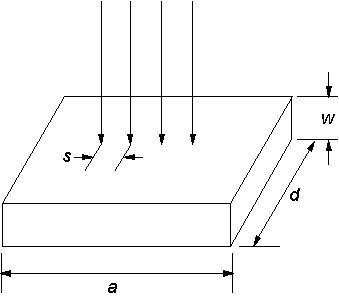
Figure 3.12. Schematic diagram of four-point probe measurements of a thin wafer.

 

The sheet resistance of a thin wafer, i.e. w much smaller than either a or d, is given by Equation 3.5, and has units of W/square.

 

                                       Equation 3.5

The correction factor, CF, is obtained from a calibration graph of d/s vs CF, as given in Figure 3.13.

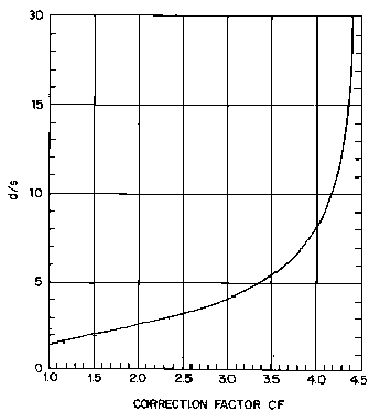
Figure 3.13. Calibration graph of d/s vs correction factor, for measurement of sheet resistance using a four‑point probe (adapted from reference [[6]]).

 

Resistivity is given by Equation 3.7 in which w is the film thickness (cm), thus yielding a resistivity with units of W cm.

 

                                             Equation 3.7

 

Four sets of V/I data were taken for each film.  After the first reading the probes were lifted off the film surface before being replaced for the second reading.  The probes were then rotated through 90º prior to the third measurement, before again being lifted and repositioned for the final reading.  This procedure produced four values of R_s, which were then averaged before the final conversion to resistivity.  This process obtained an average resistivity independent of probe orientation. 

 

3.4. Optical Emission Spectroscopy

 

Optical emission from the plasma exited the deposition chamber through a quartz viewport before being focused into a quartz fibre-optic bundle (see Figure 3.14).  The light was then dispersed, using an Oriel InstaSpec 77480 spectrometer (600 lines/mm grating and 50 mm slit), before being directed onto an Oriel InstaSpec IV charged coupled device (CCD) array (1024 pixels).  In such a way, a spectrum covering a 300 nm wavelength range can be imaged in one measurement. 

 

(c)

(d)

(b)

(a)

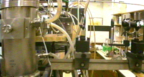
Figure 3.14. OES experimental apparatus showing (a) reactor chamber view‑port, (b) focusing lens, (c) iris and (d) fibre-optic mount.

 

Every spectrum was accumulated using 1000 exposures, each of 0.1 s duration.  The wavelength scale was manually calibrated using the emission from room lights, an example spectrum is given in Figure 3.15.  Light was sampled from the centre of the plasma ball with a spatial resolution of ~3 mm, and a spectral resolution ≤0.3 nm, over the wavelength range being investigated (~200-520 nm).  It should be noted that no corrections were made to the spectra for the wavelength dependent optical response of the fibre-optic, spectrometer or CCD array.

 

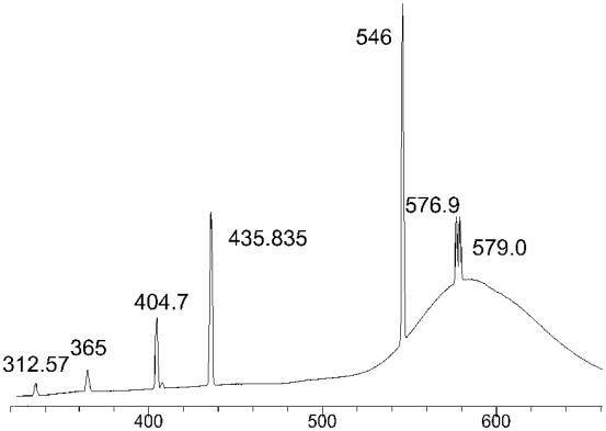
Wavelength ¾®

 

Figure 3.15. Emission spectrum from room lights, used to calibrate OES wavelength scale.  Numbers on the various peaks refer to wavelength of Hg emission lines (in nm).

 

3.5. Molecular Beam Mass Spectroscopy (MBMS)

 

This section deals with the system used to sample gas from, and analyse the species present in, microwave plasma and hot filament activated diamond CVD gas mixtures.  The mass spectrometer apparatus is identical to that used during previous studies undertaken in Bristol investigating both hot filament [[7]-[8][9][10][11][12]] and microwave plasma [1,[13],[14]] diamond CVD.  A thorough description of the apparatus is given in Reference 1, however a more general treatment will be given in this section.

 

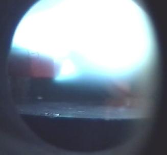
Figure 3.16. Photograph taken through chamber viewport showing gas sampling from the side of a 50%CH₄/50%CO₂ microwave plasma ball.  The molybdenum tip of the stainless steel sampling probe is seen to glow red hot.

 

3.5.1. Gas Sampling From Plasma Ball

 

Gas was sampled from the side of the microwave plasma ball via an orifice (~100 mm diameter) in a molybdenum sampling cone (see Figure 3.16).  The extraction orifice was drilled into the centre of the cone tip using the frequency-doubled output of a Nd-YAG laser (532 nm), focused by a 20 cm focal length lens.  The cone was welded to a stainless steel sampling probe, as illustrated in Figure 3.17.  A mounting flange at the base of the probe incorporated six bolt holes, thus making it possible to mount the probe onto another flange attached to the reaction chamber (as described in Section 3.2.2).  This connection was made vacuum tight by the use of a copper gasket seal.

 

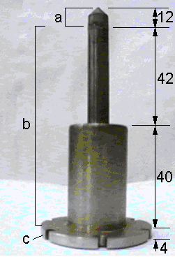
Figure 3.17. Photograph of MBMS sampling probe showing (a) molybdenum cone, (b) stainless steel tubing (2 mm thick with outside diameters of 10 and 26 mm) and (c) mounting flange (outside diameter 50 mm).  Dimensions shown are in mm.

 

3.5.2. Gas Sampling From Vicinity of Hot Filament

 

Mass spectrometric measurements of hot filament activated gas mixtures were made using the MWCVD reaction chamber.  One of the chamber windows was removed and replaced with a feedthrough flange.  This allowed a variac power supply to be connected to a pair of tungsten rods within the chamber.  Thus, power was supplied to a coiled filament, positioned 5 mm from the sample probe orifice.  The filament was prepared by winding a length of Ta wire (0.25 mm-thick) into a coil with diameter of ~4 mm and length ~1 cm.  Six turns of the wire was the standard used in all hot filament experiments.  A schematic diagram of the experimental apparatus is given in Figure 3.18.

 

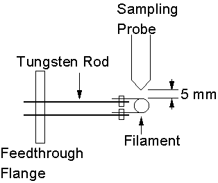
Figure 3.18. Schematic diagram of hot filament placement within MWCVD chamber.  The diagram presents a top view of the apparatus.

 

3.5.3. MBMS First Stage

 

Gas passing through the sampling cone orifice entered the first stage differential pumping chamber (components shown in red in Figure 3.2).  During experimental measurements the first stage was maintained at a pressure <10^-3 Torr by means of an Edwards 240 l/s turbomolecular pump, backed by an Edwards E2M2 two stage rotary pump.  The base pressure achievable being ~10^-7 Torr. This stage had two functions, firstly it allowed the high pressure (~20 Torr) reaction chamber to be coupled to a mass spectrometer, which had to be maintained at pressures of ~1×10^-6 Torr.  Secondly, the large pressure drop (>20000 times) experienced by gas passing from the plasma into the first stage led to adiabatic expansion and the formation of a molecular beam. 

3.5.4. MBMS Second Stage

 

The molecular beam entered the mass spectrometer second stage via a 1 mm skimmer orifice.  During experimental measurements the skimmer was located ~10 cm behind the orifice in the sampling cone.  However, the entire molecular beam mass spectrometer was mounted on a rail, with flexible exhaust connections between the turbomolecular and rotary pumps.  This enabled the second stage to be retracted away from the sampling orifice, and through a set of bellows, to a position behind a gate valve.  Thus, it was possible to isolate the two molecular beam mass spectrometer stages from the reaction chamber, allowing vacuum to be maintained within the former during regular venting of the latter.  An Edwards 70 l/s turbomolecular pump backed by an Edwards E2M1.5 two stage rotary pump evacuated the second stage.  This achieved base and operational pressures of 5×10^-8 and ~1×10^-6 Torr, respectively.  The back flange of the second stage incorporated a vacuum feedthrough for the RF power supply and electronics associated with the quadrupole mass spectrometer, QMS, (a Hiden Analytical HAL/3F PIC 100).

 

3.5.5. Considerations for MBMS studies

 

The signal intensity of a species Y, I(Y), is related to the mole fraction of Y present in the CVD chamber, X(Y), by the following relationship:

 

I(Y) = S_ms × S_exp × X(Y)                                               Equation 3.7

 

where S_ms and S_exp are sensitivity factors for Y.  S_ms accounts for the effects of mass spectrometer detection (Section 3.6) and therefore is dependent on the electron ionisation cross section of Y (at a given ionising electron energy, e),  in addition to the efficiency of the transport of Y⁺ through the quadrupole mass filter, and its subsequent detection.  These factors are intrinsic to Y and did not vary during the duration of a MBMS experiment.  However, S_exp deals with the effects of gas mixture transport through the expansion, and therefore varied with the local temperature, pressure and composition of the gas sample.  It is consequently of great importance to understand the behaviour of S_exp.

 

Studies [8] using the same MBMS apparatus as discussed here have shown that the amount of a pure gas (e.g. H₂, Ar) flowing into the mass spectrometer (proportional to the mass spectrometer signal) varied as T_gas^-0.6.  It was also found that when using a mixture of a “heavy” inert gas diluted in a lighter carrier gas (e.g. 2% Ar/H₂) the Ar signal was proportional to T_gas^-1.6.  This highlights an additional effect, that of mass dependent thermal diffusion, which depletes the sampling region of heavy gas species.  

 

3.6. Hiden Analytical HAL/3F PIC Quadrupole Mass Spectrometer

 

The vacuum components of the QMS are contained within the second differential pumping stage.  These consist of a Source, Quadrupole mass filter and Detector.  These components are shown in Figure 3.19 and are discussed in the following sections.

 

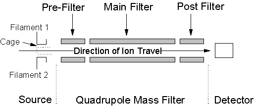
Figure 3.19. Diagram of the mass spectrometer vacuum components, showing the Source, Quadrupole mass filter and Detector.

 

3.6.1. Source

 

The source region consists of two tungsten filaments (F1 and F2) arranged around a wire mesh cage.  Electrons produced via thermionic emission from the filaments are accelerated to a user-defined energy (0-150 eV) by a voltage applied to the cage.  The species within the molecular beam are ionised by these electrons before proceeding into the quadrupole mass filter.  It should be noted that the electrons are produced with a distribution of energies (FWHM = 0.5 eV).

 

 

 

 

3.6.2. Quadrupole Mass Filter

 

As its name suggests, the quadrupole mass filter consists of four metal electrodes ~6 mm in diameter, and approximately 20 cm in length.  The rods are parallel and arranged in a square, with opposite pairs of electrodes being electrically common.  Voltages, with both d.c and RF components, are applied to the opposing pairs of electrodes.  Ions moving through the mass filter follow oscillating paths, caused by the time dependent electric fields induced by the biased electrodes.  Such ion trajectories may be resonant (in which case the ion will pass through the mass filter), or non-resonant (meaning that the ion will oscillate away from the centreline and be lost at an electrode).  Which path an ion with a given mass-to-charge ratio, m/q, follows is determined by the RF and d.c voltages applied to the electrodes.  Therefore, it is possible to filter out all but one ion mass (i.e. m/q ratio) from the molecular beam and, by using pre-set voltage settings, a complete mass spectrum (m/q = 1-100) can be collected.

 

3.6.3. Detector

 

Ions allowed to pass through the mass filter travel on to the continuous dynode secondary electron multiplier.  Secondary electrons are created when ions collide with the detector.  These secondary electrons are accelerated by a high applied voltage before again colliding with the detector and liberating more electrons.  In such a manner a cascade is set up, allowing a huge gain (~10⁷), thus producing a measurable current from each ion impact.

 

3.6.4. HAL/3F PIC 100 QMS: System Control Unit

 

A microprocessor unit controls the mass spectrometer components allowing data to be collected in histogram form (BAR mode) or as a table of up to 16 ion counts (Multiple Ion Detection, MID, mode).  Full descriptions of the computerised operating system are given in References 1 and [15], therefore only system settings utilised for the collection of experimental results presented in this thesis are given, in Table 3.2.

 

Parameter	Description	Settings used in work presented
DISCRM	Noise discriminator level	0 to –20%
DELTAM	Mass filter resolution at low masses	0 to –20%
RES’N	Mass filter high mass resolution	0 to –40%
SEM	Secondary Electron Multiplier applied voltage	2500 kV
ENERGY	Ionising electron energy	Species dependent (see Section 3.7.2)
CAGE	Source cage voltage	3.0 V
EMISS	Emission current of ionising electrons	120 mA
DWELL	Acquisition time for each ion	200 ms

Table 3.2. Typical mass spectrometer operating parameters used in the present work.

 

3.7. Mass Spectrometer Characterisation

 

As discussed earlier, gas molecules present within the molecular beam are ionised by electrons produced by the mass spectrometer ioniser filaments.  For this to happen, the kinetic energy of the ionising electron must be sufficient to remove an electron from the molecule in question.  The minimum energy required is the molecule’s ionisation potential, IP, a parameter that varies for different species.  Therefore, for a species Y to be ionised, an ionisation electron is required of energy, e, that is greater than IP(Y).  Thus:

 

Y + e^- → Y⁺ + 2e^-                    (e ≥ IP(Y) eV)                         Reaction 3.1

 

3.7.1. Energy Scale Calibration

 

The energy scale of the electrons produced by filaments 1 and 2 (F1 and F2) has previously been calibrated against the first ionisation potential of Ar (i.e. 15.76 eV) [1,11].  These studies have shown that, while F1 generates electrons of the same energy set by the control box, the energy of electrons produced by F2 is in fact 2 eV lower than that set.  Therefore, all the MBMS results presented in the following chapters were collected using F1.

 

3.7.2. Threshold Ionisation Technique

 

If the ionising electron has sufficient energy, a molecule it encounters may not only become ionised, but also dissociated.  The threshold for this dissociative ionisation of molecule Z, to produce Y⁺, is termed the appearance potential of Y, AP(Y⁺ from Z).  For example, IP(CH₃) = 9.84 eV [[16]], but at ionisation electron energies, e, greater than the AP(CH₃⁺ from CH₄) of 14.3 eV [16], CH₃⁺ will arise from the “cracking” of CH₄.  This means that measured signal counts for CH₃⁺ made at ionisation electron energies greater than 14.3 eV will arise from both CH₃ originating from the CVD reaction chamber, and dissociative ionisation of CH₄ occurring within the mass spectrometer. As a consequence, measurements of CH₃ must be made at an energy that is above 9.84 eV yet below 14.3 eV.  In practice, measurements of CH₃ were all made at an electron ionisation energy of 13.6 eV.  This energy is sufficiently higher than IP(CH₃), to obtain significant signal counts, and lower than AP(CH₃⁺ from CH₄), to minimise signal due to cracking of CH₄.  The use of such electron ioniser settings is termed the threshold ionisation technique [[17]].

 

3.8. MBMS Experimental Procedure

 

This section outlines the use of the molecular beam mass spectrometer to make measurements of a microwave plasma.  The specific example of studying the effect of H₂S addition to a 1% CH₄/H₂ gas mixture, at 20 Torr, is given here.  However, the data collection procedure is identical for studies of hot filament activated gas mixtures.  It should be noted that this general method was not always practical, as explained in Section 3.11.

 

1. Prior to starting an experiment, the mass spectrometer ioniser filament should have been left on for at least 5 days prior to the experiment (see Reference 1).
2. The reaction chamber Edwards E2M40 rotary pump should have evacuated all gas lines back to the cylinder taps (usually overnight).
3. The gate valve can then be opened and the MBMS second stage wound forward into position. 
4. The species and mass spectrometer parameters relevant to the experiment are entered into the mass spectrometer system control unit (MID mode).  Pressing HT ON then activates the detector.  Pressing START begins the display of species detected counts. 
5. The H₂ background signal for the reactor chamber is measured.
6. The vacuum seal between the sample probe and the MBMS first stage is now checked.  This is done by introducing H₂ into the reactor chamber.  An MBMS second stage pressure below ~2×10^-6 Torr, for a reactor chamber pressure of 20 Torr, is indicative of a good seal [1].
7. Background signals for all species of interest (except H₂) are measured, at a chamber pressure of 20 Torr and room temperature.  These are checked for ~1 hour to ensure they remain steady over time.
8. The H₂ is evacuated from the chamber.
9. The initial experimental gas flow of 1% CH₄/H₂ is set and the mixture is introduced to the CVD chamber at 20 Torr. 
10. A room temperature calibration for CH₄ is now obtained, by measuring the signal for 1% CH₄ and H₂ (both at 16.0 eV).  Cracking of CH₃ from CH₄ is possible, so the CH₃ signal (at 13.6 eV) must also be measured, to find out how much CH₃ signal due to cracking is related to the signal for 1% CH₄.  Again these measurements are checked for stability with time. 
11. The plasma is now struck and left to equilibrate for 30 minutes, at the experimental conditions (1000 W applied microwave power). 
12. Mass spectroscopic analysis of species signal is now carried out as described in Section 3.9.
13. H₂S is introduced into the reactor chamber and the plasma is again left (30 minutes) to equilibrate.  Species signals are taken before the next H₂S addition concentration is set. 
14. Step 13 is repeated for H₂S additions over the range 1000-10000 ppm. 
15. The H₂S supply is then shut off and the plasma is left to equilibrate until negligible counts of H₂S are measured (~1 hour).
16. Measurements of all species counts are then made, in order to check any trends observed during the course of the experiment.
17. The plasma is switched off and the apparatus is allowed to cool down to room temperature. 
18. The gases are evacuated from the reactor, and 1% of each stable species in H₂ is fed into the CVD chamber at 20 Torr.  The calibration signals representing 1% of each stable species are measured.  Possible cracking product signals are also recorded.  The calibrations must be performed on the same day as the mass spectrometric experiment to ensure the results are not affected by sensitivity changes of the mass spectrometer with time.
19. The mass spectrometer is then retracted and the gate valve closed.  All gas supplies are shut off, and lines are left pumping back to the gas cylinder taps.
20. Experimental data is fed into an Excel computer spreadsheet program, which undertakes the data corrections laid out in Section 3.10 to yield species mole fractions.

 

3.9. Mass spectrometric Data Collection

 

Detected counts were read off the MBMS system control box display and manually entered into a scientific calculator (in statistics mode).  The number of readings taken was between 10 and 20.  The mean and standard deviation of the data were then computed.  This procedure was used to collect all data presented in the following chapters, except in the case discussed in Section 3.11.2.

 

3.9.1. Notation

 

For the remainder of this thesis such averaged mass spectroscopic signal counts for species Y will be denoted I(Y) (e.g. I(CH₄) refers to averaged counts of CH₄).  The subscript ‘BG’ will indicate a background measurement, e.g. I_BG(CH₄).  In this instance the measurement is made prior to the experiment at the process pressure and room temperature, using a feed gas of 100% H₂ (i.e. step 7 in Section 3.8).  One exception is the background counts of H₂, denoted I_BG(H₂),  The measurement of which was made with the reactor chamber evacuated (i.e. step 5 in Section 3.8).  The subscript ‘TCORR’ denotes a signal that has been scaled to yield a room temperature measurement, and has also been background corrected.  A signal that has also been corrected for cracking effects is given the subscript ‘CORR’.  The subscript ‘CAL Y’ is used for a signal measured during calibration of Y, i.e. for a 1% dilution of Y in H₂, at process pressure and room temperature, step 18 in Section 3.8.

 

3.10. Data Analysis Procedure

 

The following Section describes the procedure by which measured species counts are converted into species mole fractions.  This procedure is identical to that used during previous Bristol investigations [1] of MWCVD.  The overview of the conversion is as follows.  Firstly, signals are scaled, from the values measured at T_gas ~ 1600 K, to magnitudes predicted at room temperature.  Further corrections are then carried out for the effects of background due to species present in the CVD chamber and cracking of species inside the mass spectrometer. The corrected counts are then converted to mole fractions using room temperature calibration measurements of stable species.  It should be noted that this procedure was only possible for studying H₂S additions to 1% CH₄/H₂ gas mixtures, as discussed in Section 3.11.1. 

 

3.10.1. Temperature and Background Correction

 

The signal counts measured for species sampled from the plasma (T_gas ~1600 K) are smaller in magnitude than those measured in 20 Torr of H₂.  This is due to the temperature dependence of the gas flow through the sampling orifice.  Therefore, prior to calibration against room temperature counts of stable species, these signals must be scaled to yield room temperature measured counts.  Since the CVD mixture is almost 100% H₂, the flow of the gas mixture through the sampling orifice can be assumed to be dominated by the flow properties of H₂ [1,11].  The H₂ signal is then used to rescale all measured counts (for a specific set of conditions), relative to a background corrected measurement of H₂ signal made using a 1% CH₄/H₂ gas mixture at room temperature, I_RT(H₂).  Following further subtraction of background signals (measured at room temperature), temperature corrected signals (I_TCORR(Y)) are obtained.

 

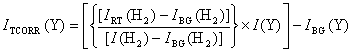        Equation 3.8

 

3.10.2. Correction for Cracking Products

 

As mentioned previously (Section 3.7.2), signals arising from cracking products can contribute to the mass spectrometer signal for a particular species.  Although the threshold ionisation technique minimises such problems, they are not entirely eliminated.  Therefore, it is necessary to include an additional correction to the species signals affected.  Consider the situation of a species Y being studied at an ionising electron energy, e_Y, such that dissociative ionisation of species Z also produces Y⁺.  When a room temperature calibration of Z is performed, the Y⁺ signal is also measured (at e_Y).  The signal corrected for cracking products is denoted I_CORR(Y), thus:

 

               Equation 3.9

 

The subscript ‘CAL Z’ indicates that I(Y) and I(Z) were measured during the calibration of Z.

 

3.10.3. Room Temperature Species Calibration

 

Stable species calibration was carried out at room temperature, by introducing a known amount (usually 1% in H₂) of each stable species, X(Y), into the CVD chamber, at the process pressure of 20 Torr.  The signal for the species is then recorded and background corrected, thus a room temperature calibration is obtained which connects a mole fraction of species present in the CVD chamber to a MBMS signal measurement.  The temperature corrected experimental species counts can then be ratioed to this calibration.  Room temperature calibrations are carried out, once the apparatus has cooled down, and on the same day as experimental measurements.  In such a way mole fractions for stable species are obtained.  Thus,

 

                                   Equation 3.10

 

Note that, if no correction for cracking is needed, I_TCORR(Y) is used in place of I_CORR(Y).  Also, as X(Y) = 1%, the final species mole fraction will be in units of %.

 

3.10.4. Calibration of Radical Species

 

Direct calibration of free radical species is not possible, therefore an indirect calibration method is needed.  The present work includes measurements of the radical species CH₃ and CS.  A calibration for CH₃ was developed during previous studies of HFCVD at Bristol [9,11], and has since been applied to MWCVD investigations [1]. The procedure calculates the measured counts, I_{CAL Y} (Y), arising from a theoretical room temperature calibration for a 1% dilution of the radical species in H₂.  Here Y refers to either the CH₃ or CS radical_. 

 

                                 Equation 3.11

 

where I_CAL Z (Z) is the calibration counts for a species, Z, related to Y (e.g. CH₄ or CS₂).  Q(Y) and Q(Z) are the ionisation cross sections of Y and Z, measured at e_Y and e_Z.  P corresponds to the partitioning of counts due to Y present in the molecular beam and Y present in the background gas within the mass spectrometer.  Previous work has determined this background partitioning factor for CH₃ (P = 0.35), and this value has also been used to calibrate the CS radical.  Values of Q(Y) and Q(Z), along with literature references, are presented in Table 3.3.

 

 

Species Y	CH3	CS
Species Z	CH4	CS2
eY	13.6 eV	13.6 eV
eZ	16.0 eV	16.0 eV
Q(Y)	0.26 Å2 (Reference [18])	0.88 Å2 (Reference [19])
Q(Z)	0.22 Å2 (Reference [20])	2.75 Å2 (Reference 19)

Table 3.3. Parameters required for the calculation of calibration signals for CH₃ and CS.

 

The values of I_{CAL Y} (Y) calculated are then used to convert I(Y) into X(Y), using Equation 3.10.

 

3.11. Problems encountered during MBMS investigations

 

This section will deal with the problems encountered while attempting to make mass spectrometric measurements of microwave plasma activated CH₄/CO₂ gas mixtures.  Underlying difficulties concerning the study of such gas mixtures are discussed first, before more specific problems related to investigations of CH₄/CO₂ mixing ratios, and H₂S additions to 51%CH₄/49%CO₂ gas mixtures.  It should also be noted that although all deposition experiments were carried out at a pressure of 40 Torr, mass spectroscopic measurements for all gas mixtures, except binary CH₄/CO₂ gas mixtures, were only possible at 20 Torr.  This was due to plasma instability observed at higher pressures.

 

3.11.1. Species Mole Fraction Calibration for CH₄/CO₂ Gas Mixtures

 

The fundamental problem concerning these gas mixtures is that mass spectrometric signal counts cannot be calibrated to yield species mole fractions.  Such a calibration requires knowledge of the temperature dependent transport properties of species passing through the sampling orifice.  In the case of gas mixtures that are almost completely composed of H₂, such species properties are dominated by those of H₂ (Section 3.10.1).  Therefore, this type of calibration can be undertaken for investigation of small (~1%) H₂S additions to 1% CH₄/H₂ (see Chapter 6).  However, such an assumption cannot be made when looking at mixtures of CH₄ and CO₂.  As a result, no quantitative comparisons of species counts will be made, and the quoted magnitude of signal counts should be treated with caution.  Instead, the present work will concentrate on comparisons of the trends observed in measured species counts over the range of CH₄/CO₂ gas mixtures investigated.

 

3.11.2. Investigations of CH₄:CO₂ Mixing Ratios

 

It was found that the MBMS source cage became coated with an insulating layer of material (probably diamond-like carbon) when using methane rich process gas (e.g. >60% CH₄).  This resulted in a medium term drift in ionisation efficiency, and therefore signal levels, for measurements made after such deposition has occurred.  Such an effect is evident in Figure 3.20, where signal counts for a number of species are seen to drop over time, for a 50%CH₄/50%CO₂ gas mixture maintained at a constant pressure (40 Torr).

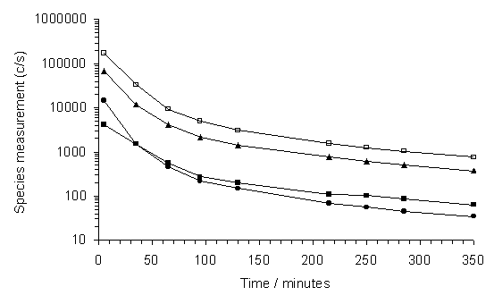
Figure 3.20. Species signal counts measured for a 50%CH₄/50%CO₂ gas mixture, following measurements being made of high CH₄ content gas mixtures.  Conditions: MW applied power 1000 W, pressure 40 Torr, ionising electron energy 20 eV.  Key: (<) H₂, (▲) CH₃, (ÿ)CH₄, (·) CO₂.

 

It was therefore necessary to measure all the species, at all mixing ratios of interest (100%CO₂-80%CH₄/20% CO₂), in as short a time as possible.  In practice, each process gas mixture was allowed to stabilize for ~2 minutes before the entire mass spectrum (m/z = 0-100) was then printed, before moving on to the next gas mixture.  Species measured signal counts were then read off the resulting histograms.  No further problems of this kind were observed after the final high %CH₄ measurement had been made, and the source cage having been cleaned.

 

3.11.3. Investigations of H₂S Addition to 51%CH₄/49%CO₂ Gas Mixtures

 

The MBMS apparatus was modified during the period prior to the study of these gas mixtures being undertaken.  The entire second stage mass spectrometry apparatus was removed and left at atmosphere for four months, while the work presented in Appendix 1 was carried out.  When the apparatus was reassembled it was discovered that a significant background was present, over the entire spectrometer range (m/z = 0‑100).  Despite numerous attempts to find the cause, no solution was found to this problem. 

 

However, as stated already, MBMS measurements of species present in CH₄/CO₂ CVD gas mixtures cannot be converted to mole fractions.  Therefore, the absolute magnitude of raw species signals are unimportant, as only data trends are to be investigated.  The presence of significant background counts was therefore ignored.  This was much less of a problem in the case of the S-containing species investigated, with low counts of these species detected in plasmas with no sulfur addition.  These counts were therefore treated as background and subtracted off the species dataset.  After species measurements were made for the final H₂S addition (1%), the sulfur supply was shut off and the plasma was left for ~1 hour.  Further species measurements were then undertaken and compared with those taken prior to any H₂S addition.  Data for any species whose measured counts failed to revert to those seen initially were disregarded.  The observed trends for such species counts are assumed to be the result of fluctuations in the background.

 

3.12. References