The Self-Consistent Field (SCF) Method

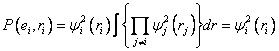
Simply, to calculate a potential energy surface, we must solve the electronic Schrödinger equation (equations (3.3)—(3.5)) for a system of n electrons and N nuclei, over a range of nuclear coordinates. This is termed an ab intio method, since it is derived from ‘first principles’.

Generally, the real wavefunction of a system is too complex to be found directly, but can be approximated by a simpler wavefunction. This then enables the electronic Schrödinger equation to be solved numerically. The self-consistent field method is an iterative method that involves selecting an approximate Hamiltonian, solving the Schrödinger equation to obtain a more accurate set of orbitals, and then solving the Schrödinger equation again with theses until the results converge.

7.1 Hartree-Fock theory

The Hartree-Fock (HF) method [14],[15] invokes what is known as the (molecular) orbital approximation: The wavefunction is taken to be a product of one-electron wavefunctions (equation (7.1)):

(7.1)

These one-electron wavefunctions are also called orbitals. In the case of a molecule, the orbitals are expanded as atomic functions, according to a basis set:

(7.2)

The molecular orbital approximation assumes that the electrons behave independently of each other (equation (7.3) shows that the probability density for an electron does not depend on other electrons), and that the electronic Hamiltonian can be expressed as a sum of one-electron Hamiltonians (equation (7.4)).

(7.3)

(7.4)

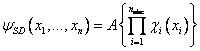
The wavefunctions are written as antisymmetrised products of spin-orbitals (equations (7.5) and (7.6), where SD denotes that the wavefunction is written as a Slater determinant (see Levine[7])) in order to satisfy the Pauli principle, since the Hartree method does not ordinarily account for spin.

(7.5)

(7.6)

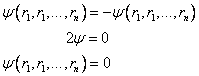
Pauli showed that relativistic quantum field theory indicates that particles with half-integral spin (e.g. s=½), such as electrons, require antisymmetric wavefunctions:

(7.7)

In spin-orbital terms, if two electrons have the same spin, the wavefunction becomes zero. E.g. If r₁ = r₂ in equation (7.7):

(7.8)

The continuous nature of (7.8) means that the probability of finding two electrons with the same spin close to each other is very small. See Levine[7] or Szabo and Ostlund[16] for a greater discussion of the Pauli principle.

The Hartree-Fock energy is given from the energy of the Slater determinant, by equation (7.9):

(7.9)

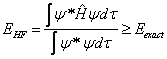
In order to find the best wavefunction, the variational method is used. This relies on the variational principle, that the approximate Hartree-Fock wavefunction is always greater in energy than the exact ground state energy of the system (equation (7.10) – the complex conjugate of the wavefunction is multiplied by the wavefunction (integrated over all space) to normalise the probability density (recall equation (2.13))).

(7.10)

The energy of the Hartree-Fock wavefunction depends on the atomic orbital coefficients, c_ij, (equation (7.2)) used in the linear combination of atomic orbitals to construct the molecular wavefunction (orbital).
The variational method, then, involves choosing these coefficients so as to minimise the energy (equation (7.11)):

(7.11)

Being an SCF method, the Hartree-Fock method then uses this wavefunction again to construct another, until the energies converge.
The variational method is discussed in most physical chemistry text books that cover quantum chemistry, but this Adobe Acrobat file at the University of Missouri-Rolla is a useful resource for those looking on the web.

7.2 Perturbation theory

An alternative to the variational theorem used to minimise the energy of the Slater determinant coefficients in the Hartree-Fock method is perturbation theory. This is discussed in detail in Levine[7] and Szabo and Ostlund,[16] but is simply the fact that an approximation to an unsolvable Hamiltonian lies in a simpler Hamiltonian (the example given in Levine is the case of harmonic and anharmonic oscillators). The simpler Hamiltonian (superscript zero in equation (7.12), below) is called the unperturbed system, and the more accurate Hamiltonian the perturbed system. The difference between the two is the perturbation, often denoted by a prime:

(7.12)

7.2.1 Møller-Plesset (MP) perturbation theory

A common form of so-called many-body perturbation theory is Møller-Plesset (MP) perturbation theory, formulated in 1934 by Møller and Plesset.[17] In MP theory, the HF wavefunction is the unperturbed system.
Various levels of MP theory exist, each offering a greater correction to the Hartree-Fock energy, the most commonly used being MP2:

(7.13)

…where E⁽¹⁾ and E⁽²⁾ denote first- and second-order corrections to the zeroth-order (unperturbed) wavefunctions.
MP calculations are much faster than configuration interaction (CI) calculations (see section 8) and go some way to correcting for electron correlation effects, but are not variational methods and so can produce an energy below the true wavefunction energy.
MP calculations are, however, useful for excited state configurations, where the variation method (HF) fails.

7.2.2 Coupled-cluster (CC) perturbation theory

Another popular perturbation correction method is the coupled-cluster (CC) method, (also termed the coupled-cluster approximation (CCA)) suggested in 1958 by Coester and Kümmel.[18],[19] Originally suggested for problems in nuclear physics, this was applied to the quantum chemistry many-body problem by Cízek.[20]
The method is based on a set of couple equations for the one-, two-, three-, … particle cluster functions, and it can be shown that this set of “coupled cluster” equations is equivalent to the Schrödinger equation for the many particle system (Mezey[21]).
Coupled-cluster theory is also discussed in Levine.[7]

7.3 The Multi-Configuration Self-Consistent Field (MCSCF) Method

The multi-configuration SCF (MCSCF) method involves choosing non-SCF molecular orbitals and varying these so as to minimise the energy. The molecular wavefunction is again written as a linear combination of the configuration state functions, varying the coefficients and also the forms of the molecular orbitals.
The advantage of the MCSCF method is that the non-SCF molecular orbitals may provide faster convergence to the exact wavefunction than SCF molecular orbitals, which in turn means fewer configuration state functions need to be included in the wavefunction. The amount of calculation involved in MCSCF calculations is great, but it is still a widely used method.
The MCSCF method is also detailed in Szabo and Ostlund.[16]

7.4 The Complete Active Space Self-Consistent Field (CASSCF) Method

The most commonly used form of MCSCF calculations is the complete active space SCF (CASSCF) method.
In this situation, the orbitals used in the configuration state functions are divided into active and inactive orbitals. The inactive orbitals are doubly occupied in all configuration functions; electrons not in inactive orbitals are called active electrons.
The wavefunction is written as a linear combination of the configuration functions that can be formed by distributing the active electrons amongst the active orbitals in all permutations corresponding to the same spin and symmetry as the state being calculated. Most often, the active orbitals are the valence orbitals.
CASSCF is reasonably accurate and frequently used. It is outlined in more detail in this paper.[22]