|
|
||||||||||||||||
World of Colour
|
The physical measurement of colour | |
Measuring Concentrations using absorbance, | |
Transition Metal Solutions, |
Rhodopsin and the eye
Basics behind Dyes and Pigments
Phosphorescence and Fluorescence
A Thermochromic example
Colour Therapy
Detection using Optical Sensors
Symbols, Glossary, Disclaimer, Credits, References, feedback..
Action 3: Book turning. This image is taken from gifs (ref. 14) and is copyright restricted according to the source given (i.e. it is not the authors' own work).
|
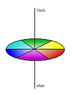
The physical measurement of colour: The primary colours are those that cannot be made by the mixing of other colours and yet between them make up all the colours of the spectrum. Red, blue and green are known as the additive primaries but yellow is thought of as the third primary instead of green in most contexts. There are three properties of colour that need to be considered:
reflected.
Figure 2: Colour wheel. The idea for this image is taken from Christie (ref. 3) and is copyright restricted according to the source given (i.e. it is not the author’s own work). Using the colour wheel given, all three attributes can be quantified: the hue is within the plane of the colour wheel itself; the chroma increases with distance from the centre; and the lightness is the third dimension with black (no light reflected) and white (all light reflected) as the extremes.
|
| Transition metal solutions: Why
are they so colourful? The non-degeneracy of the five 3d orbitals in
transition metal complexes is governed by their dissimilar orientations:
the 2 “axial” orbitals (d(x2–y2) and d(z2)
– i.e. those pointing directly at the ligands) are relatively de-stabilised
compared to the 3 other orbitals (d(xy), d(xz) and d(yz)) which point
between them. This is explained fully in the Crystal Field Theory of
transition metal complexes and also has great bearing on what is currently
under discussion. For example, Titanium
(III) is a colourless gas as a free ion however, due to an electronic d-d
transition between the two now, non-degenerate d-orbital sets, the Ti3+
hexaaqua
complex appears as a deep purple solution. Remember, objects which are exposed
to white light appear coloured as they have absorbed the energy
corresponding to the wavelength of the complimentary colour.
Other transition metal solutions are different colours due to
the variation of Δoct which is itself dependent on the nature of the ligands within the complex. Simply
click on the empty beaker below to see just a few transition metal
solutions:
Action 5: Some typical transition metal solution
|