Addition Rule

Differentiate all adding terms sequentially, and add the results together.

Examples

1. y = 3x² + 2x + 7, = 6x + 2

2. p = 9m - 2m³, = 9 - 6m²

3. y = mx + c, = m (as we saw before).

4. φ = 14λ² - + λ³ + 3, = 28λ - 2λ⁹ + 3λ²

5. p(T) = (at constant n, R, V),

Negative powers of x

Recall that we can have negative powers of x as well, i.e.

x^-1 = ,        x^-2 =

and in general, x^-n =

These, too, obey the general 'magic' formula:

Examples

1. y = = 5x^-1, = -5x^-2 = -

2. y = = 3x^-2 - , = -6x^-3 + = -

3. V(r) = - (= the potential between 2 electrons at a separation of r)

= (= the force of repulsion between them - the famous inverse square law)

Roots - Fractional powers of x

Square roots, cube roots, fourth roots, etc., can all be represented as fractional powers of x.

e.g. = x^½ , = x^1/3

= x^2/3 , 1 / = x^-½

= (x + 1)^½ , 1 / = (x² + 3)^-1/3

These, too, obey the magic formula.

Examples

1. y = = x^½ , = ½ x^-½ =

2. y = = x^2/3 , = =

3. y = 1 / = x^-½ , = -½ x^-3/2 = -

4. φ(λ) = - = λ^½ - 3λ^-3/2,

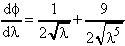
Now we have a method to calculate the value of a slope at any point along a curve, without having to draw the graph and construct the tangent.

Examples

1. What is the gradient of y(x) = x² - 4x - 1 at the point x = 4? (Note: this is the same function we solved graphically, earlier)

Gradient = = 2x - 4

so, when x = 4, = (24) - 4 = 4 (as we found before)

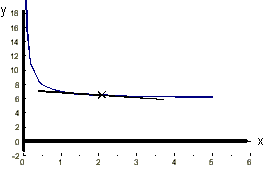
2. What is the gradient of y(x) = + 6 at the point x = 2?

= -

so when x = 2, = - ¼

3. What is the gradient of p(q) = - 2q² at q = 3?

= q² - 4q, so when q = 3, = - 3

Zero gradients Turning points, maxima and minima

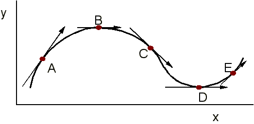
Consider a function which gives a curve like that above. If we measure the gradient at different points we get different answers:

at points A and E gradient is +ve

at point C gradient is -ve

So at some points in between, B and D, the function exhibits a stationary value, and this can either be a local maximum (B) or local minimum(D).

The points at which a curve exhibits a maximum or minimum are very important in chemistry since this often indicates when the behaviour of a system changes, shows where an equilibrium position lies, or shows where something is most (or least) probable.

How do we calculate maxima and minima positions?

We know that at a local max or min, the gradient = 0, i.e. dy/dx = 0. So, given a function, y(x), all we need to do is differentiate it, and put the derivative equal to zero, then solve for x.

Examples

1. y(x) = x³ - 3x + 1

= 3x² - 3

When = 0, then 3x² - 3 = 0

3x² = 3

x² = 1

x = +/- 1

when x = +1, y = -1

when x = -1, y = 3

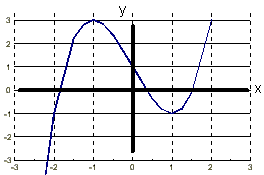
(Note: later we'll show how we tell which is a max and min).

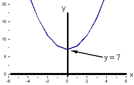
2. y = x² + 7

= 2x

At stationary point, = 0,

so 2x = 0, i.e. x = 0 and y = 7.

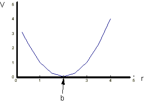
3. The potential V of a diatomic molecule (e.g. Cl₂) can be approximated by a quadratic function of the bond length, r, of the form:

V(r) = k(r - b)² [k and b are constants]

What is the equilibrium bond length?

Answer : Multiplying out: V(r) = kr² - 2kb.r + kb²

The equilibrium position will occur when the potential changes from attractive to repulsive, i.e. when the slope changes from +ve to -ve, e.g. at the minimum value of V.

So we need = 0,

= 2kr - 2kb = 0

r = b

So the constant b is actually the equilibrium bond length. The value of V at which this occurs is V(b) = 0.