Molecular Dynamics Simulations

· To begin, require atomic coordinates and velocities:

· Generate ‘start-up’ configuration – all atoms assigned positions, r_i, and velocities v_i.

· Velocities chosen appropriate to a particular temperature (e.g. 300K) – see below

· Given potential function V(r), calculate forces as:

F = -dV(r)/dr

Solve Newton’s equations of motion:

F_i=m_ia_i

or d²r_i/dt² = F_i/m_i

To obtain dynamic behaviour, need to solve 2^nd order differential equation for every particle in the system

r_i(t+Dt) = r_i(t) +v_iDt + 1/2a_i(Dt)² + …

Typically, Leapfrog Verlet method used, with timestep (Dt) approx. 1fs (10^-15s)

r_i(t+Dt) = r_i(t) +v(t–Dt/2) + m_i^–1F_i(t)Dt

v_i(t+Dt/2) = v_i(t –Dt/2) + m_i^–1F_i(t)Dt

So the positions of the atoms, and their velocities at a susbsequent time t+Dt can be found. This procedure is repeated thousands of times to allow equilibration, and obtain an equilibrium distribution of velocities.

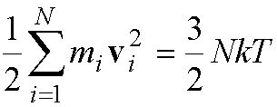
Unlike Monte Carlo, the temperature of the system is typically not fixed. The temperature of the system can be calculated from the kinetic energy of all the N atoms:

· Special techniques may be needed to ensure that the temperature does not change too far from the desired simulation temperature (e.g. by scaling velocities).

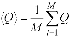
· Properties (e.g. thermodynamic averages) can be calculated from a molecular dynamics simulation by a time average of the values for the configurations generated in the simulation:

where M is the number of time steps.

Molecular dynamics simulations are used for the same type of systems as Monte Carlo – they have been particularly useful for proteins and polymers, where it may be difficult to design good Monte Carlo moves. Molecular dynamics simulations are very important in the study of protein folding.

Comments on the Monte Carlo and molecular dynamics simulation methods

· Obvious difference: molecular dynamics provides information on time-dependence of properties, Monte Carlo does not.

· Typical conditions for dynamics simulation: constant number of particles (N), constant volume (V), constant energy (E), the NVE or ‘microcanonical’ ensemble.

· Typical conditions for Monte Carlo simulation: constant number of particles (N), constant volume (V) and constant temperature (T), the NVT or ‘canonical’ ensemble.

· MD has a kinetic energy contribution, in MC the total energy is just calculated from the potential function

· Monte Carlo and molecular dynamics simulations are good for disordered systems, such melts, liquids, solutions (in comparison with lattice dynamics which is good for solids (ordered)).

· It is difficult to model rare events (e.g. crossing barriers from one state to another) as high energy configurations (e.g. transition states) are sampled only rarely. Techniques such as ‘umbrella sampling’ are used to force a system to change from one state into another (e.g. to force a chemical reaction to occur in a QM/MM simulation). A ‘biasing’ potential forces the system to move along a reaction coordinate to the transition state, and then to the products.

· The calculation of absolute free energies is very difficult with either method. However, the convergence of the ensemble averages is very slow. Instead, relative free energies can be calculated by gradually (and non-physically) ‘mutating’ one structure into another in a series of simulations, for example in the free energy perturbation technique. One amino acid sidechain could be mutated into another in a series of simulations to find the effect on a protein.