Quantum Wave Mechanics – The Schrödinger Equation

2.1 The time-dependent Schrödinger equation

Classical mechanics uses deterministic equations to define the state and motion of a macroscopic system at a given point. According to Newton’s second law (equation (2.1)), the future state and motion of a system can be exactly determined, given the state of the system at any time - an example of this is given in Levine.[7]

(2.1)

For a microscopic particle, Heisenberg’s uncertainty principle shows that we cannot know the exact position and velocity of a particle at a specific simultaneous point in time – this means classical mechanics cannot be used to predict the state and motion of microscopic – or quantum – particles.
To describe the state of a quantum mechanical system, a function of the particles’ coordinates called the wavefunction, or state function, is used. This is a corollary of the wave-particle duality of quantum particles – that if a particle with a fixed momentum has a fixed wavelength, then it must be possible to represent it mathematically as a wave, that is, by using a wavefunction. In classical physics, a steady wave motion of wavelength l propagating in the positive x-direction is represented by equation (2.2):

(2.2)

…where i represents the square root of –1.
Since the state of a quantum particle typically changes with time, the wavefunction, Ψ, is also a function of time. For a one-particle, one-dimensional system, Ψ = Ψ(x,t).
The equation describing how a wavefunction changes with time was discovered in 1926 by the physicist Erwin Schrödinger,[8] and is presented for a one-particle one-dimensional system in equation (2.3):

(2.3)

…where m is the mass of the particle, V(x,t) is the potential energy function of the system, i again represents the square root of –1, and the constant ħ is defined as in equation (2.4):

(2.4)

Equation (2.3) is known as the time-dependent Schrödinger (wave) equation. It represented the start of Schrödinger’s work into quantum wave mechanics, most notably for proving that matrix mechanics (treating the electron as a quantum particle, the work of Heisenberg) and wave mechanics (treating the electron as a wave) were compatible. He was jointly awarded the Nobel Prize for Physics in 1933 with Paul Dirac for this work (Dirac for his work on electron and positron theory).
The time-dependent Schrödinger equation enables the calculation of the future wavefunction (or state) of the system at any time, provided the wavefunction at a time t₀ is known.
Quantum mechanics is statistical in nature, in that it can only provide probabilities of properties such as the location of a particle, and not a definitive answer.
In a light beam, the wavefunction is spread out evenly over the whole wave front, but when photons are detected, on a fluorescent screen for example, they arrive at unpredictable locations with a probability density proportional to the intensity of the light beam, or the square of the wave amplitude.
Max Born suggested that this might also be the case for particles represented by wavefunctions. He postulated that the probability of finding a particle in the interval region between x and x+dx, where that particle is represented by the wavefunction Ψ(x,t), is that given in equation (2.5):

(2.5)

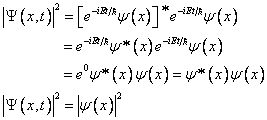
…where Ψ* represents the complex conjugate of Ψ.
The function |Ψ(x,t)|² is known as the probability density of the wavefunction, for finding the particle at various positions along the x-axis.

2.2 The time-independent Schrödinger equation

In chemistry, the simpler time-independent Schrödinger equation is more often used than the time-dependent Schrödinger (equation ((2.3)). This is derived from the time-dependent version by considering the special case where the potential energy, V, is a function of only position, x and not of time, t. Solutions of (2.3) that can be written as a product of a function of time and a function of x:

(2.6)

Partial derivation of (2.6) gives:

(2.7)

Which, upon substitution into the time-dependent Schrödinger equation, (2.3), gives:

(2.8)

…which is divided by fΨ:

(2.9)

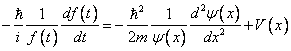
Each side of (2.9) is expected to be a function of x and of t. The right side, however, does not depend on t, and so is independent of it. Similarly, the left side is independent of x. Since the function is independent of both variables, x and t, it must be a constant. This is called E. Equating the right side of (2.9) to E gives:

(2.10)

This is the time-independent Schrödinger equation for a single particle of mass m moving in one dimension. E has the same units as V, and is therefore postulated to be the energy of the system.
Equating the left side of (2.10) to E produces a function for f(t):

(2.11)

This then means that where the potential energy is a function of x only, wavefunctions of the following form exist:

(2.12)

The probability density function can be shown to be time-independent thus:

(2.13)

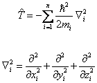
2.3 The three-dimensional many-particle Schrödinger equation

The time-independent Schrödinger equation is often represented as energy eigenfunctions and eigenvalues, using the Hamiltonian operator, Ĥ:

(2.14)

For a one-particle, three-dimensional system, the classical-mechanical Hamiltonian is as given in equation (2.15):

(2.15)

Quantum-mechanically, this is represented as in equation (2.16):

(2.16)

…where the section in parentheses is called the Laplacian operator, Ñ ² (equation (2.17)).

(2.17)

The three-dimensional, one-particle time-independent Schrödinger equation is thus represented as in equation (2.18):

(2.18)

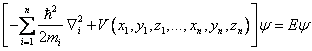
A many particle system can be represented by considering a system of n particles, where particle i has mass m_i and spatial coordinates (x_i, y_i, z_i), where i=1,2,3,…,n.
Classically, the total kinetic energy is the sum of the kinetic energies of the individual particles. Quantum-mechanically, the kinetic energy operator is that in equation (2.19):

(2.19)

The potential energy is usually only taken to be dependent on the 3n spatial coordinates. The time-independent Schrödinger equation then becomes:

(2.20)