Molecular Simulation – continued

Leach, Chapter 6 (and 7 & 8); Grant and Richards Chapter 4

Monte Carlo (MC) and Molecular Dynamics (MD)

These are the two most common simulation methods in molecular modelling.

Boundary conditions

· Even with approximate methods, cannot simulate very large numbers of atoms.

· Get round this by using periodic boundary conditions (as shown previously for lattice dynamics) – the simulation system is replicated in all directions, and interacts with its ‘images’, giving a pseudo-infinite system.

· Alternatively, can focus on just a small region of a large molecule, and using some boundary restraints at the edges to make sure the structure is maintained, and the effects of the environment are included approximately.

Monte Carlo

To calculate a particular property, Q, of a system with a constant number of particles, temperature and volume (the NVT or canonical ensemble): statistical mechanics shows that the average value of Q, <Q> is given by:

P(X) is the Boltzmann weighted probability:

where U(X) is the internal energy (e.g. calculated by molecular mechanics) and X represents all possible configurations of the system.

· You might have thought the values of these integrals could be found by simply sampling different configurations of the system by moving atoms at random, calculating the value of Q(X) at each configuration, and averaging to get <Q>.

· However, this wouldn’t work – each configuration would make the same contribution, whereas in fact the probability term means that only configurations with low energies make a significant contribution to P(X).

· The correct way to do the sampling of configurations is to use the Metropolis method: in this the generation of configurations is biased towards those that make the most important contributions.

· Specifically, configurations are generated with a Boltzmann probability exp(-U(X)/kT.

· So the Monte Carlo method generates configurations randomly and uses a specific set of criteria (usually the Metropolis method) to decide whether or not to accept each new configuration.

· These criteria ensure that the probability of obtaining a given configuration is equal to its Boltzmann factor exp (-U(X)/kT).

· U(X) would be calculated by molecular mechanics, for example.

· Configurations with low energy are generated with higher probability than configurations with higher energy.

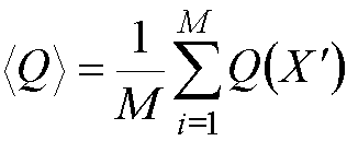
For each configuration that is accepted, the values of the desired properties are calculated, and at the end of the calculation, the average of these properties is obtained by simply averaging over the number of configurations, M:

where X' indicates that only configurations with an acceptable Boltzmann weighted probability have been sampled. (Q could be for example the internal energy, calculated as the average of the energies of the configurations generated in the simulation).

In a Monte Carlo simulation, each new configuration of the system is generated by a random move of an atom or molecule, or (in the case of large molecules such as polymers or proteins) by more sophisticated ‘moves’, such as rotation around bonds or concerted motions. The energy, U(X), is calculated for the new configuration.

Then

· If the energy of the new configuration is lower than the energy of its predecessor, the new configuration is accepted.

· If the energy of the new configuration is higher than the energy of its predecessor, then the Boltzmann factor of the energy difference is calculated: exp (-DU/kT). The Boltzmann factor is compared with a random number between 0 and 1. If the random number is lower than the Boltzmann factor, the new configuration is accepted and the configuration is included. If the random number is higher, then the new configuration is rejected, and the original configuration is used for the next iteration

· This procedure allows moves to states of higher energy. The smaller the increase in energy (DU), the greater the probability that the configuration will be accepted.

Monte Carlo simulations are used for simulations of liquids, solids, solutions, polymers, proteins, etc.

Next: molecular dynamics simulations