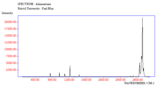
Fig.19. The full range Raman spectrum of adamantane, as displayed on a web page using Chime and JCAMP data.
Scientific reports often need to display spectral information from a wide variety of sources, such as infrared absorption, optical emission, nuclear magnetic resonance, electron spin resonance, etc. However, traditionally, the only way to incorporate spectral data into a paper was a simple 2D graph, which often had to be printed on a small scale due to size restrictions in the Journals. That meant that important information within the spectra was often unreadable. But now that many papers are being published in electronic format, it's possible to include a lot more of the spectral information alongside the actual spectra itself.
Probably the best example of spectral data format this is the Joint Committee on Atomic and Molecular Physical data extension (JCAMP-DX) file, which is a way of formatting spectral data in terms of x,y coordinates. Many spectrometers can now export their data files directly into JCAMP format. Specialised graphical viewers (such as JCAMP data viewer) have been developed which can then display these files at a later date, and manipulate them offline. For example, the spectra can be expanded or shrunk, viewed on different scales, and the exact position of peaks and troughs can be determined.
JCAMP files are given the extrension .jdx, and an example of such a file can be seen below.
<##TITLE= Simplified IR Spectrum of water
##JCAMP-DX= 4.24 $$ Written by Drive for Windows v 1.39
##DATA TYPE= SPECTRUM
##ORIGIN= Gaussian 94 Frequencies
##OWNER= P.W. May
##XUNITS= Wavenumber (CM^-1)
##YUNITS = Intensity (Arb. Units)
##PEAK ASSIGNMENT= (XYWA)
##NPOINTS=822
##XYDATA=(X+(Y..Y))
500,-0.0001
501,-0.0002
502,-0.0002
503,-0.0003
504,-0.0002
505,-0.0003
[...many points removed for brevity]
4498,0.0000
##END=
The ## signs signify a comment, and these lines give extra information about how the spectrum was created (either experimentally or in simulation), and by whom. The main data can be formatted in a number of different styles, and in this case the attribute ##XYDATA=(X+(Y..Y)) defines it as a series of increasing x,y data points, which then follow as a set of comma-separated pairs on separate lines. More information about the exact specification for the contents and attributes of JCAMP files can be found in Ref.[12] .
JCAMP format is, of course, ideal for use in internet Journals, and the Chime plug-in has been extended to act as an online JCAMP viewer. The only extra code that needs to be added to include the JCAMP data on a web page is:
<embed src="adamantane.jdx" width="90%" height="90%">
where src specifies the path to and name of the file containing the JCAMP data, and the other parameters specify the display size on the screen.
The spectrum appears directly on the web page with a large degree of interactivity. By clicking on a peak, the x,y, coordinates of that point are displayed. Also, by selecting regions of interest by drawing a box around them with the mouse cursor, the spectrum can be zoomed to look at parts of the spectrum in more detail. An example of a JCAMP spectrum for the laser Raman spectrum of adamantane is shown in Fig.19, as it would appear on a web page, and in expanded form in Fig.20. If you have the Chime plug-in, you can see this in action for yourself by clicking here.
Fig.19. The full range Raman spectrum of adamantane, as displayed on a web page using Chime and JCAMP data.

Fig.20. By zooming into the structure around 2900 cm-1, more detail can be displayed.
One of the most exciting things that can be done with JCAMP spectra is to link them to 3D molecular structures. For example, we can display the infrared absorption spectrum of water alongside the 3D molecule, and when the user clicks on particular peaks in the spectrum an animation initiates showing the vibrational mode of water which caused the chosen absorption peak. The first requirement, of course, is that the animations have been previously assigned, and created as xyz files, using the methods detailed previously in section (d). In the case of water, we require 4 separate xyz files, one for each of the 3 distinct vibrational modes, and one for 'off', i.e. when the user clicks on a part of the spectrum not containing a peak.
The spectrum and 3D structure files can be displayed on the web page alongside each other using table formatting:
<table align=center>
<tr>
<td><embed src="h2o.jdx" width=400 height=300><td>
<td><embed src="h2ovib.0.xyz" name="CHIMEDISP" frank=false width=200 height=200 animfps=10 animmode=loop script="zoom 180; rotate y 90; wireframe 40; spacefill 100">><td>
</tr>
</table>
As before, the 'src' parameter defines the path and name of the JCAMP file (h2o.jdx). The second line is for the 3D structure display, which begins with the static display (h2ovib.0.xyz). The following CHIME parameters then give the display a name (CHIMEDISP), so that the JCAMP file will know which file on the page to interact with, as well as setting up the default display characteristics. The result looks like the image given in Fig.21.
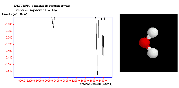
Fig.21. The appearance on a web page of the JCAMP infrared spectrum of water alongside its 3D structure.
To make the spectrum interact with the 3D structure file, it is necessary to add some extra information to the JCAMP file. The required lines are:
##$ASSIGNMENT TYPE=CHIME
##$CHIME TARGET=CHIMEDISP
##PEAK ASSIGNMENT= (XYWA)
2170,-1,25, <load "h2ovib.1.xyz"; select *; zoom 180; rotate y 90; wireframe 40; spacefill 100; animation on; select hydrogen; wireframe off">
4141,-1,25, <load "h2ovib.2.xyz"; select *; zoom 180; rotate y 90; wireframe 40; spacefill 100; animation on; select hydrogen; wireframe off">
4393,-1,25, <load "h2ovib.3.xyz"; select *; zoom 180; rotate y 90; wireframe 40; spacefill 100; animation on; select hydrogen; wireframe off">
2250,-1,1750, <load "h2ovib.0.xyz"; select *; zoom 180; rotate y 90; wireframe 40; spacefill 100">
The parameter 'ASSIGNMENT TYPE' defines that the file will interact with a Chime file, and the 'CHIME TARGET' parameter defines which of the possible Chime structures on the web page is to be affected when the user clicks on particular parts of the spectrum, by referring to the 'NAME' it was given earlier. The lower four lines then define the special regions of the spectrum, 'hot-spots', which when activated cause affects to be visible in the 3D window. The three numbers refer to the x coordinate position at the centre of the hot-spot, (e.g. 2170), the y coordinate position (-1 means all y values are accepted), and the tolerance on the x values (e.g. 25 means within 25 units of the central x coordinate). The subsequent Chime script then tells the file how to behave if the user clicks within the hot-spot - in this case it should 'load' a new xyz file with the specified display characteristics and begin the animation. Subsequent lines define other 'hotspots' in the spectrum with their related xyz files. The last line defines the default stationary image for the case where a user clicks outside any of the hot-spots.
If you have the Chime plug-in, you can see this in action by clicking on the hyperlink for the file h2o.htm. Other examples of linking JCAMP spectra and Chime animations can be seen in one of our recent papers [13] and at Robert Lancashire's site at the University of the West Indies [14]. Interactive spectra linking to normal mode vibrations can also be visualised with the ComSpec VRMl applet from the University of Erlangen [10].